---
blogpost: true
date: Jun 20, 2019
title: Load Large Image Data with Dask Array
author: John Kirkham
tags: python, scipy, scikit-image, dask-image
---

## Executive Summary

This post explores simple workflows to load large stacks of image data with Dask array.

In particular, we start with a [directory full of TIFF
files](https://drive.google.com/drive/folders/13mpIfqspKTIINkfoWbFsVtFF8D7jbTqJ)
of images like the following:

```
$ $ ls raw/ | head
ex6-2_CamA_ch1_CAM1_stack0000_560nm_0000000msec_0001291795msecAbs_000x_000y_000z_0000t.tif
ex6-2_CamA_ch1_CAM1_stack0001_560nm_0043748msec_0001335543msecAbs_000x_000y_000z_0000t.tif
ex6-2_CamA_ch1_CAM1_stack0002_560nm_0087497msec_0001379292msecAbs_000x_000y_000z_0000t.tif
ex6-2_CamA_ch1_CAM1_stack0003_560nm_0131245msec_0001423040msecAbs_000x_000y_000z_0000t.tif
ex6-2_CamA_ch1_CAM1_stack0004_560nm_0174993msec_0001466788msecAbs_000x_000y_000z_0000t.tif
```

and show how to stitch these together into large lazy arrays
using the [dask-image](https://image.dask.org/en/latest/) library

```python
>>> import dask_image
>>> x = dask_image.imread.imread('raw/*.tif')
```

or by writing your own Dask delayed image reader function.

<table>
<tr>
<td>
<table>  <thead>    <tr><td> </td><th> Array </th><th> Chunk </th></tr>
  </thead>
  <tbody>
    <tr><th> Bytes </th><td> 3.16 GB </td> <td> 316.15 MB </td></tr>
    <tr><th> Shape </th><td> (2010, 1024, 768) </td> <td> (201, 1024, 768) </td></tr>
    <tr><th> Count </th><td> 30 Tasks </td><td> 10 Chunks </td></tr>
    <tr><th> Type </th><td> uint16 </td><td> numpy.ndarray </td></tr>
  </tbody></table>
</td>
<td>
<svg width="176" height="181" style="stroke:rgb(0,0,0);stroke-width:1" >

  <!-- Horizontal lines -->
  <line x1="10" y1="0" x2="80" y2="70" style="stroke-width:2" />
  <line x1="10" y1="61" x2="80" y2="131" style="stroke-width:2" />

  <!-- Vertical lines -->
  <line x1="10" y1="0" x2="10" y2="61" style="stroke-width:2" />
  <line x1="17" y1="7" x2="17" y2="68" />
  <line x1="24" y1="14" x2="24" y2="75" />
  <line x1="31" y1="21" x2="31" y2="82" />
  <line x1="38" y1="28" x2="38" y2="89" />
  <line x1="45" y1="35" x2="45" y2="96" />
  <line x1="52" y1="42" x2="52" y2="103" />
  <line x1="59" y1="49" x2="59" y2="110" />
  <line x1="66" y1="56" x2="66" y2="117" />
  <line x1="73" y1="63" x2="73" y2="124" />
  <line x1="80" y1="70" x2="80" y2="131" style="stroke-width:2" />

  <!-- Colored Rectangle -->
  <polygon points="10.000000,0.000000 80.588235,70.588235 80.588235,131.722564 10.000000,61.134328" style="fill:#ECB172A0;stroke-width:0"/>

  <!-- Horizontal lines -->
  <line x1="10" y1="0" x2="55" y2="0" style="stroke-width:2" />
  <line x1="17" y1="7" x2="62" y2="7" />
  <line x1="24" y1="14" x2="69" y2="14" />
  <line x1="31" y1="21" x2="77" y2="21" />
  <line x1="38" y1="28" x2="84" y2="28" />
  <line x1="45" y1="35" x2="91" y2="35" />
  <line x1="52" y1="42" x2="98" y2="42" />
  <line x1="59" y1="49" x2="105" y2="49" />
  <line x1="66" y1="56" x2="112" y2="56" />
  <line x1="73" y1="63" x2="119" y2="63" />
  <line x1="80" y1="70" x2="126" y2="70" style="stroke-width:2" />

  <!-- Vertical lines -->
  <line x1="10" y1="0" x2="80" y2="70" style="stroke-width:2" />
  <line x1="55" y1="0" x2="126" y2="70" style="stroke-width:2" />

  <!-- Colored Rectangle -->
  <polygon points="10.000000,0.000000 55.850746,0.000000 126.438982,70.588235 80.588235,70.588235" style="fill:#ECB172A0;stroke-width:0"/>

  <!-- Horizontal lines -->
  <line x1="80" y1="70" x2="126" y2="70" style="stroke-width:2" />
  <line x1="80" y1="131" x2="126" y2="131" style="stroke-width:2" />

  <!-- Vertical lines -->
  <line x1="80" y1="70" x2="80" y2="131" style="stroke-width:2" />
  <line x1="126" y1="70" x2="126" y2="131" style="stroke-width:2" />

  <!-- Colored Rectangle -->
  <polygon points="80.588235,70.588235 126.438982,70.588235 126.438982,131.722564 80.588235,131.722564" style="fill:#ECB172A0;stroke-width:0"/>

  <!-- Text -->

<text x="103.513608" y="151.722564" font-size="1.0rem" font-weight="100" text-anchor="middle" >768</text>
<text x="146.438982" y="101.155399" font-size="1.0rem" font-weight="100" text-anchor="middle" transform="rotate(-90,146.438982,101.155399)">1024</text>
<text x="35.294118" y="116.428446" font-size="1.0rem" font-weight="100" text-anchor="middle" transform="rotate(45,35.294118,116.428446)">2010</text>
</svg>

</td>
</tr>
</table>

Some day we'll eventually be able to perform complex calculations on this dask array.

<img src="https://raw.githubusercontent.com/mrocklin/raw-host/gh-pages/images/aollsm-index-1.jpg"
     width="45%"
     alt="Light Microscopy data rendered with NVidia IndeX">
<img src="https://raw.githubusercontent.com/mrocklin/raw-host/gh-pages/images/aollsm-index-2.jpg"
     width="45%"
     alt="Light Microscopy data rendered with NVidia IndeX">

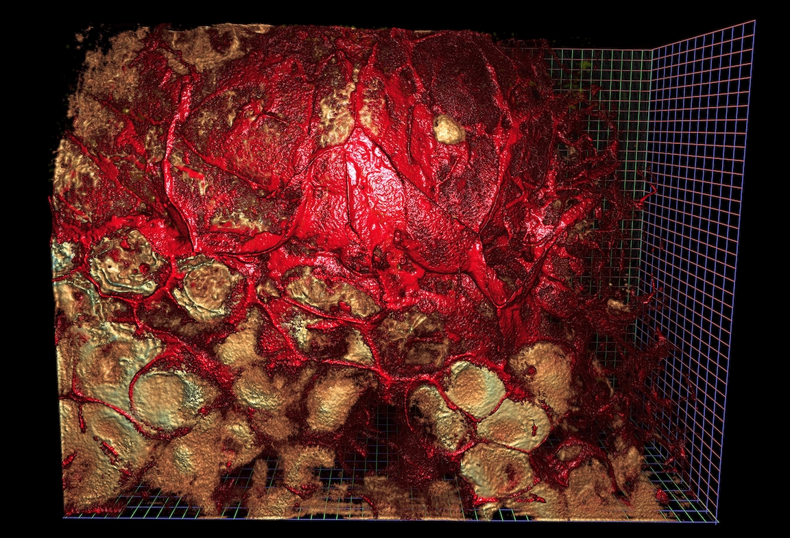
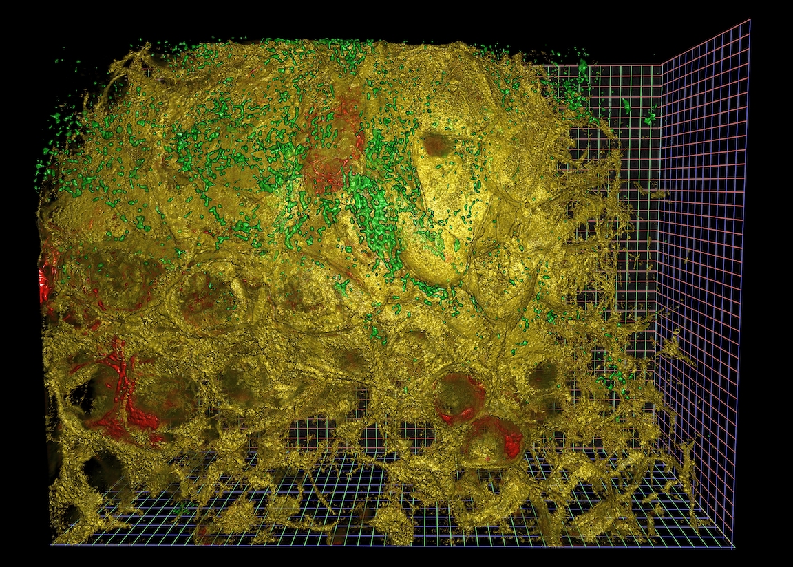
_Disclaimer: we're not going to produce rendered images like the above in this
post. These were created with [NVidia
IndeX](https://developer.nvidia.com/index), a completely separate tool chain
from what is being discussed here. This post covers the first step of image
loading._

## Series Overview

A common case in fields that acquire large amounts of imaging data is to write
out smaller acquisitions into many small files. These files can tile a larger
space, sub-sample from a larger time period, and may contain multiple channels.
The acquisition techniques themselves are often state of the art and constantly
pushing the envelope in term of how large a field of view can be acquired, at
what resolution, and what quality.

Once acquired this data presents a number of challenges. Algorithms often
designed and tested to work on very small pieces of this data need to be scaled
up to work on the full dataset. It might not be clear at the outset what will
actually work and so exploration still plays a very big part of the whole
process.

Historically this analytical process has involved a lot of custom code. Often
the analytical process is stitched together by a series of scripts possibly in
several different languages that write various intermediate results to disk.
Thanks to advances in modern tooling these process can be significantly
improved. In this series of blogposts, we will outline ways for image
scientists to leverage different tools to move towards a high level, friendly,
cohesive, interactive analytical pipeline.

## Post Overview

This post in particular focuses on loading and managing large stacks of image
data in parallel from Python.

Loading large image data can be a complex and often unique problem. Different
groups may choose to store this across many files on disk, a commodity or
custom database solution, or they may opt to store it in the cloud. Not all
datasets within the same group may be treated the same for a variety of
reasons. In short, this means loading data is a hard and expensive problem.

Despite data being stored in many different ways, often groups want to reapply
the same analytical pipeline to these datasets. However if the data pipeline is
tightly coupled to a particular way of loading the data for later analytical
steps, it may be very difficult if not impossible to reuse an existing
pipeline. In other words, there is friction between the loading and analysis
steps, which frustrates efforts to make things reusable.

Having a modular and general way to load data makes it easy to present data
stored differently in a standard way. Further having a standard way to present
data to analytical pipelines allows that part of the pipeline to focus on what
it does best, analysis! In general, this should decouple these to components in
a way that improves the experience of users involved in all parts of the
pipeline.

We will use
[image data](https://drive.google.com/drive/folders/13mpIfqspKTIINkfoWbFsVtFF8D7jbTqJ)
generously provided by
[Gokul Upadhyayula](https://scholar.google.com/citations?user=nxwNAEgAAAAJ&hl=en)
at the
[Advanced Bioimaging Center](http://microscopy.berkeley.edu/)
at UC Berkeley and discussed in
[this paper](https://science.sciencemag.org/content/360/6386/eaaq1392)
([preprint](https://www.biorxiv.org/content/10.1101/243352v2)),
though the workloads presented here should work for any kind of imaging data,
or array data generally.

## Load image data with Dask

Let's start again with our image data from the top of the post:

```
$ $ ls /path/to/files/raw/ | head
ex6-2_CamA_ch1_CAM1_stack0000_560nm_0000000msec_0001291795msecAbs_000x_000y_000z_0000t.tif
ex6-2_CamA_ch1_CAM1_stack0001_560nm_0043748msec_0001335543msecAbs_000x_000y_000z_0000t.tif
ex6-2_CamA_ch1_CAM1_stack0002_560nm_0087497msec_0001379292msecAbs_000x_000y_000z_0000t.tif
ex6-2_CamA_ch1_CAM1_stack0003_560nm_0131245msec_0001423040msecAbs_000x_000y_000z_0000t.tif
ex6-2_CamA_ch1_CAM1_stack0004_560nm_0174993msec_0001466788msecAbs_000x_000y_000z_0000t.tif
```

### Load a single sample image with Scikit-Image

To load a single image, we use [Scikit-Image](https://scikit-image.org/):

```python
>>> import glob
>>> filenames = glob.glob("/path/to/files/raw/*.tif")
>>> len(filenames)
597

>>> import imageio
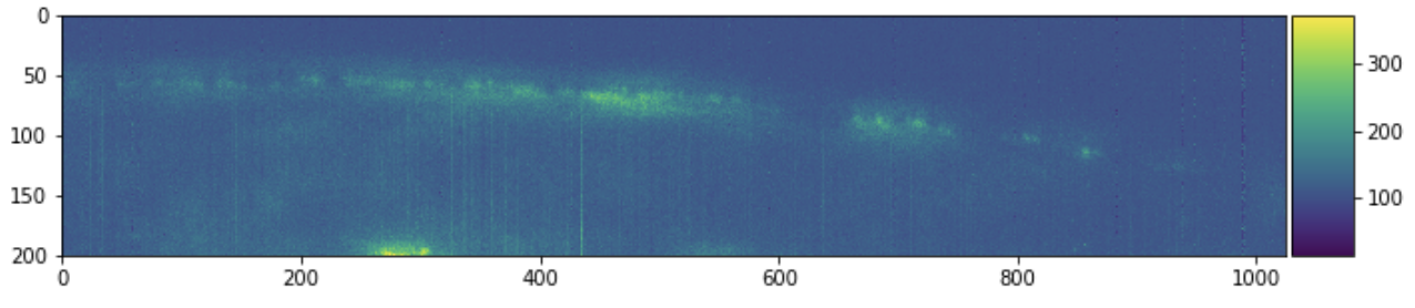
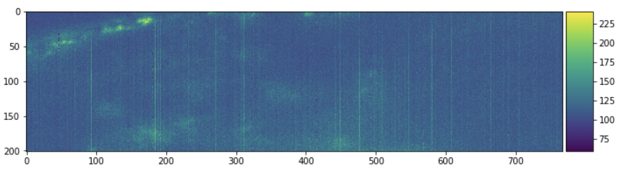
>>> sample = imageio.imread(filenames[0])
>>> sample.shape
(201, 1024, 768)
```

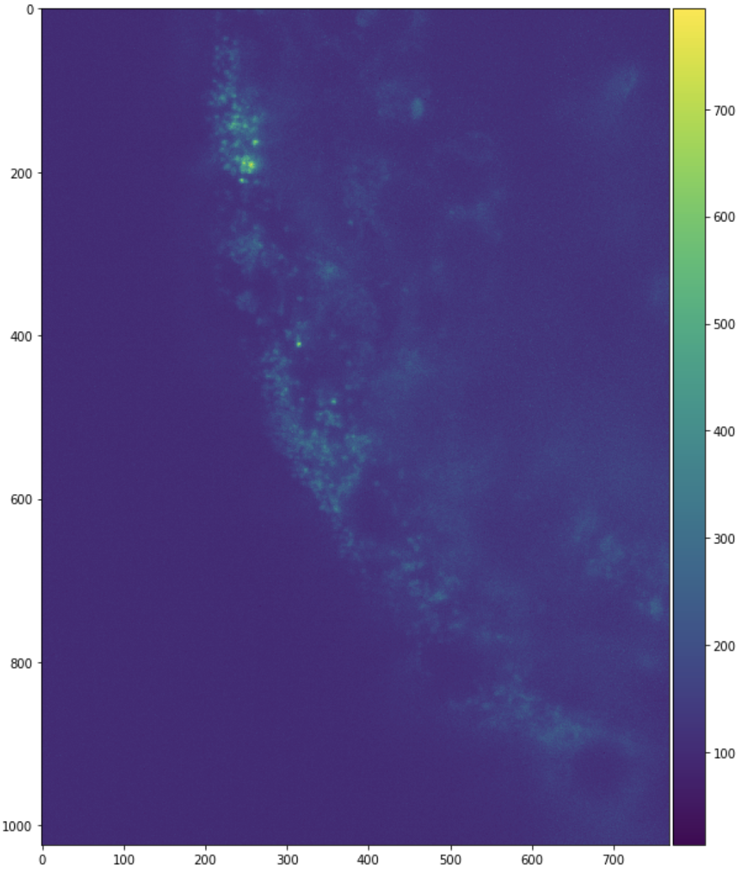
Each filename corresponds to some 3d chunk of a larger image. We can look at a
few 2d slices of this single 3d chunk to get some context.

```python
import matplotlib.pyplot as plt
import skimage.io
plt.figure(figsize=(10, 10))
skimage.io.imshow(sample[:, :, 0])
```

<img src="https://raw.githubusercontent.com/mrocklin/raw-host/gh-pages/images/aollsm-sample-1.png"
     width="60%">

```python
plt.figure(figsize=(10, 10))
skimage.io.imshow(sample[:, 0, :])
```

<img src="https://raw.githubusercontent.com/mrocklin/raw-host/gh-pages/images/aollsm-sample-2.png"
     width="60%">

```python
plt.figure(figsize=(10, 10))
skimage.io.imshow(sample[0, :, :])
```

<img src="https://raw.githubusercontent.com/mrocklin/raw-host/gh-pages/images/aollsm-sample-3.png"
     width="60%">

### Investigate Filename Structure

These are slices from only one chunk of a much larger aggregate image.
Our interest here is combining the pieces into a large image stack.
It is common to see a naming structure in the filenames. Each
filename then may indicate a channel, time step, and spatial location with the
`<i>` being some numeric values (possibly with units). Individual filenames may
have more or less information and may notate it differently than we have.

```
mydata_ch<i>_<j>t_<k>x_<l>y_<m>z.tif
```

In principle with NumPy we might allocate a giant array and then iteratively
load images and place them into the giant array.

```python
full_array = np.empty((..., ..., ..., ..., ...), dtype=sample.dtype)

for fn in filenames:
    img = imageio.imread(fn)
    index = get_location_from_filename(fn)  # We need to write this function
    full_array[index, :, :, :] = img
```

However if our data is large then we can't load it all into memory at once like
this into a single Numpy array, and instead we need to be a bit more clever to
handle it efficiently. One approach here is to use [Dask](https://dask.org),
which handles larger-than-memory workloads easily.

### Lazily load images with Dask Array

Now we learn how to lazily load and stitch together image data with Dask array.
We'll start with simple examples first and then move onto the full example with
this more complex dataset afterwards.

We can delay the `imageio.imread` calls with [Dask
Delayed](https://docs.dassk.org/en/latest/delayed.html).

```python
import dask
import dask.array as da

lazy_arrays = [dask.delayed(imageio.imread)(fn) for fn in filenames]
lazy_arrays = [da.from_delayed(x, shape=sample.shape, dtype=sample.dtype)
               for x in lazy_arrays]
```

_Note: here we're assuming that all of the images have the same shape and dtype
as the sample file that we loaded above. This is not always the case. See the
`dask_image` note below in the Future Work section for an alternative._

We haven't yet stitched these together. We have hundreds of single-chunk Dask
arrays, each of which lazily loads a single 3d chunk of data from disk. Lets look at a single array.

```python
>>> lazy_arrays[0]
```

<table>
<tr>
<td>
<table>  <thead>    <tr><td> </td><th> Array </th><th> Chunk </th></tr>
  </thead>
  <tbody>
    <tr><th> Bytes </th><td> 316.15 MB </td> <td> 316.15 MB </td></tr>
    <tr><th> Shape </th><td> (201, 1024, 768) </td> <td> (201, 1024, 768) </td></tr>
    <tr><th> Count </th><td> 2 Tasks </td><td> 1 Chunks </td></tr>
    <tr><th> Type </th><td> uint16 </td><td> numpy.ndarray </td></tr>
  </tbody></table>
</td>
<td>
<svg width="174" height="194" style="stroke:rgb(0,0,0);stroke-width:1" >

  <!-- Horizontal lines -->
  <line x1="10" y1="0" x2="34" y2="24" style="stroke-width:2" />
  <line x1="10" y1="120" x2="34" y2="144" style="stroke-width:2" />

  <!-- Vertical lines -->
  <line x1="10" y1="0" x2="10" y2="120" style="stroke-width:2" />
  <line x1="34" y1="24" x2="34" y2="144" style="stroke-width:2" />

  <!-- Colored Rectangle -->
  <polygon points="10.000000,0.000000 34.664918,24.664918 34.664918,144.664918 10.000000,120.000000" style="fill:#ECB172A0;stroke-width:0"/>

  <!-- Horizontal lines -->
  <line x1="10" y1="0" x2="100" y2="0" style="stroke-width:2" />
  <line x1="34" y1="24" x2="124" y2="24" style="stroke-width:2" />

  <!-- Vertical lines -->
  <line x1="10" y1="0" x2="34" y2="24" style="stroke-width:2" />
  <line x1="100" y1="0" x2="124" y2="24" style="stroke-width:2" />

  <!-- Colored Rectangle -->
  <polygon points="10.000000,0.000000 100.000000,0.000000 124.664918,24.664918 34.664918,24.664918" style="fill:#ECB172A0;stroke-width:0"/>

  <!-- Horizontal lines -->
  <line x1="34" y1="24" x2="124" y2="24" style="stroke-width:2" />
  <line x1="34" y1="144" x2="124" y2="144" style="stroke-width:2" />

  <!-- Vertical lines -->
  <line x1="34" y1="24" x2="34" y2="144" style="stroke-width:2" />
  <line x1="124" y1="24" x2="124" y2="144" style="stroke-width:2" />

  <!-- Colored Rectangle -->
  <polygon points="34.664918,24.664918 124.664918,24.664918 124.664918,144.664918 34.664918,144.664918" style="fill:#ECB172A0;stroke-width:0"/>

  <!-- Text -->

<text x="79.664918" y="164.664918" font-size="1.0rem" font-weight="100" text-anchor="middle" >768</text>
<text x="144.664918" y="84.664918" font-size="1.0rem" font-weight="100" text-anchor="middle" transform="rotate(-90,144.664918,84.664918)">1024</text>
<text x="12.332459" y="152.332459" font-size="1.0rem" font-weight="100" text-anchor="middle" transform="rotate(45,12.332459,152.332459)">201</text>
</svg>

</td>
</tr>
</table>

This is a lazy 3-dimensional Dask array of a _single_ 300MB chunk of data.
That chunk is created by loading in a particular TIFF file. Normally Dask
arrays are composed of _many_ chunks. We can concatenate many of these
single-chunked Dask arrays into a multi-chunked Dask array with functions like
[da.concatenate](https://docs.dask.org/en/latest/array-api.html#dask.array.concatenate)
and
[da.stack](https://docs.dask.org/en/latest/array-api.html#dask.array.stack).

Here we concatenate the first ten Dask arrays along a few axes, to get an
easier-to-understand picture of how this looks. Take a look both at how the
shape changes as we change the `axis=` parameter both in the table on the left
and the image on the right.

```python
da.concatenate(lazy_arrays[:10], axis=0)
```

<table>
<tr>
<td>
<table>  <thead>    <tr><td> </td><th> Array </th><th> Chunk </th></tr>
  </thead>
  <tbody>
    <tr><th> Bytes </th><td> 3.16 GB </td> <td> 316.15 MB </td></tr>
    <tr><th> Shape </th><td> (2010, 1024, 768) </td> <td> (201, 1024, 768) </td></tr>
    <tr><th> Count </th><td> 30 Tasks </td><td> 10 Chunks </td></tr>
    <tr><th> Type </th><td> uint16 </td><td> numpy.ndarray </td></tr>
  </tbody></table>
</td>
<td>
<svg width="176" height="181" style="stroke:rgb(0,0,0);stroke-width:1" >

  <!-- Horizontal lines -->
  <line x1="10" y1="0" x2="80" y2="70" style="stroke-width:2" />
  <line x1="10" y1="61" x2="80" y2="131" style="stroke-width:2" />

  <!-- Vertical lines -->
  <line x1="10" y1="0" x2="10" y2="61" style="stroke-width:2" />
  <line x1="17" y1="7" x2="17" y2="68" />
  <line x1="24" y1="14" x2="24" y2="75" />
  <line x1="31" y1="21" x2="31" y2="82" />
  <line x1="38" y1="28" x2="38" y2="89" />
  <line x1="45" y1="35" x2="45" y2="96" />
  <line x1="52" y1="42" x2="52" y2="103" />
  <line x1="59" y1="49" x2="59" y2="110" />
  <line x1="66" y1="56" x2="66" y2="117" />
  <line x1="73" y1="63" x2="73" y2="124" />
  <line x1="80" y1="70" x2="80" y2="131" style="stroke-width:2" />

  <!-- Colored Rectangle -->
  <polygon points="10.000000,0.000000 80.588235,70.588235 80.588235,131.722564 10.000000,61.134328" style="fill:#ECB172A0;stroke-width:0"/>

  <!-- Horizontal lines -->
  <line x1="10" y1="0" x2="55" y2="0" style="stroke-width:2" />
  <line x1="17" y1="7" x2="62" y2="7" />
  <line x1="24" y1="14" x2="69" y2="14" />
  <line x1="31" y1="21" x2="77" y2="21" />
  <line x1="38" y1="28" x2="84" y2="28" />
  <line x1="45" y1="35" x2="91" y2="35" />
  <line x1="52" y1="42" x2="98" y2="42" />
  <line x1="59" y1="49" x2="105" y2="49" />
  <line x1="66" y1="56" x2="112" y2="56" />
  <line x1="73" y1="63" x2="119" y2="63" />
  <line x1="80" y1="70" x2="126" y2="70" style="stroke-width:2" />

  <!-- Vertical lines -->
  <line x1="10" y1="0" x2="80" y2="70" style="stroke-width:2" />
  <line x1="55" y1="0" x2="126" y2="70" style="stroke-width:2" />

  <!-- Colored Rectangle -->
  <polygon points="10.000000,0.000000 55.850746,0.000000 126.438982,70.588235 80.588235,70.588235" style="fill:#ECB172A0;stroke-width:0"/>

  <!-- Horizontal lines -->
  <line x1="80" y1="70" x2="126" y2="70" style="stroke-width:2" />
  <line x1="80" y1="131" x2="126" y2="131" style="stroke-width:2" />

  <!-- Vertical lines -->
  <line x1="80" y1="70" x2="80" y2="131" style="stroke-width:2" />
  <line x1="126" y1="70" x2="126" y2="131" style="stroke-width:2" />

  <!-- Colored Rectangle -->
  <polygon points="80.588235,70.588235 126.438982,70.588235 126.438982,131.722564 80.588235,131.722564" style="fill:#ECB172A0;stroke-width:0"/>

  <!-- Text -->

<text x="103.513608" y="151.722564" font-size="1.0rem" font-weight="100" text-anchor="middle" >768</text>
<text x="146.438982" y="101.155399" font-size="1.0rem" font-weight="100" text-anchor="middle" transform="rotate(-90,146.438982,101.155399)">1024</text>
<text x="35.294118" y="116.428446" font-size="1.0rem" font-weight="100" text-anchor="middle" transform="rotate(45,35.294118,116.428446)">2010</text>
</svg>

</td>
</tr>
</table>

```python
da.concatenate(lazy_arrays[:10], axis=1)
```

<table>
<tr>
<td>
<table>  <thead>    <tr><td> </td><th> Array </th><th> Chunk </th></tr>
  </thead>
  <tbody>
    <tr><th> Bytes </th><td> 3.16 GB </td> <td> 316.15 MB </td></tr>
    <tr><th> Shape </th><td> (201, 10240, 768) </td> <td> (201, 1024, 768) </td></tr>
    <tr><th> Count </th><td> 30 Tasks </td><td> 10 Chunks </td></tr>
    <tr><th> Type </th><td> uint16 </td><td> numpy.ndarray </td></tr>
  </tbody></table>
</td>
<td>
<svg width="113" height="187" style="stroke:rgb(0,0,0);stroke-width:1" >

  <!-- Horizontal lines -->
  <line x1="10" y1="0" x2="27" y2="17" style="stroke-width:2" />
  <line x1="10" y1="12" x2="27" y2="29" />
  <line x1="10" y1="24" x2="27" y2="41" />
  <line x1="10" y1="36" x2="27" y2="53" />
  <line x1="10" y1="48" x2="27" y2="65" />
  <line x1="10" y1="60" x2="27" y2="77" />
  <line x1="10" y1="72" x2="27" y2="89" />
  <line x1="10" y1="84" x2="27" y2="101" />
  <line x1="10" y1="96" x2="27" y2="113" />
  <line x1="10" y1="108" x2="27" y2="125" />
  <line x1="10" y1="120" x2="27" y2="137" style="stroke-width:2" />

  <!-- Vertical lines -->
  <line x1="10" y1="0" x2="10" y2="120" style="stroke-width:2" />
  <line x1="27" y1="17" x2="27" y2="137" style="stroke-width:2" />

  <!-- Colored Rectangle -->
  <polygon points="10.000000,0.000000 27.014952,17.014952 27.014952,137.014952 10.000000,120.000000" style="fill:#ECB172A0;stroke-width:0"/>

  <!-- Horizontal lines -->
  <line x1="10" y1="0" x2="46" y2="0" style="stroke-width:2" />
  <line x1="27" y1="17" x2="63" y2="17" style="stroke-width:2" />

  <!-- Vertical lines -->
  <line x1="10" y1="0" x2="27" y2="17" style="stroke-width:2" />
  <line x1="46" y1="0" x2="63" y2="17" style="stroke-width:2" />

  <!-- Colored Rectangle -->
  <polygon points="10.000000,0.000000 46.948234,0.000000 63.963186,17.014952 27.014952,17.014952" style="fill:#ECB172A0;stroke-width:0"/>

  <!-- Horizontal lines -->
  <line x1="27" y1="17" x2="63" y2="17" style="stroke-width:2" />
  <line x1="27" y1="29" x2="63" y2="29" />
  <line x1="27" y1="41" x2="63" y2="41" />
  <line x1="27" y1="53" x2="63" y2="53" />
  <line x1="27" y1="65" x2="63" y2="65" />
  <line x1="27" y1="77" x2="63" y2="77" />
  <line x1="27" y1="89" x2="63" y2="89" />
  <line x1="27" y1="101" x2="63" y2="101" />
  <line x1="27" y1="113" x2="63" y2="113" />
  <line x1="27" y1="125" x2="63" y2="125" />
  <line x1="27" y1="137" x2="63" y2="137" style="stroke-width:2" />

  <!-- Vertical lines -->
  <line x1="27" y1="17" x2="27" y2="137" style="stroke-width:2" />
  <line x1="63" y1="17" x2="63" y2="137" style="stroke-width:2" />

  <!-- Colored Rectangle -->
  <polygon points="27.014952,17.014952 63.963186,17.014952 63.963186,137.014952 27.014952,137.014952" style="fill:#ECB172A0;stroke-width:0"/>

  <!-- Text -->

<text x="45.489069" y="157.014952" font-size="1.0rem" font-weight="100" text-anchor="middle" >768</text>
<text x="83.963186" y="77.014952" font-size="1.0rem" font-weight="100" text-anchor="middle" transform="rotate(-90,83.963186,77.014952)">10240</text>
<text x="8.507476" y="148.507476" font-size="1.0rem" font-weight="100" text-anchor="middle" transform="rotate(45,8.507476,148.507476)">201</text>
</svg>

</td>
</tr>
</table>

```python
da.concatenate(lazy_arrays[:10], axis=2)
```

<table>
<tr>
<td>
<table>  <thead>    <tr><td> </td><th> Array </th><th> Chunk </th></tr>
  </thead>
  <tbody>
    <tr><th> Bytes </th><td> 3.16 GB </td> <td> 316.15 MB </td></tr>
    <tr><th> Shape </th><td> (201, 1024, 7680) </td> <td> (201, 1024, 768) </td></tr>
    <tr><th> Count </th><td> 30 Tasks </td><td> 10 Chunks </td></tr>
    <tr><th> Type </th><td> uint16 </td><td> numpy.ndarray </td></tr>
  </tbody></table>
</td>
<td>
<svg width="197" height="108" style="stroke:rgb(0,0,0);stroke-width:1" >

  <!-- Horizontal lines -->
  <line x1="10" y1="0" x2="27" y2="17" style="stroke-width:2" />
  <line x1="10" y1="40" x2="27" y2="58" style="stroke-width:2" />

  <!-- Vertical lines -->
  <line x1="10" y1="0" x2="10" y2="40" style="stroke-width:2" />
  <line x1="27" y1="17" x2="27" y2="58" style="stroke-width:2" />

  <!-- Colored Rectangle -->
  <polygon points="10.000000,0.000000 27.988258,17.988258 27.988258,58.112379 10.000000,40.124121" style="fill:#ECB172A0;stroke-width:0"/>

  <!-- Horizontal lines -->
  <line x1="10" y1="0" x2="130" y2="0" style="stroke-width:2" />
  <line x1="27" y1="17" x2="147" y2="17" style="stroke-width:2" />

  <!-- Vertical lines -->
  <line x1="10" y1="0" x2="27" y2="17" style="stroke-width:2" />
  <line x1="22" y1="0" x2="39" y2="17" />
  <line x1="34" y1="0" x2="51" y2="17" />
  <line x1="46" y1="0" x2="63" y2="17" />
  <line x1="58" y1="0" x2="75" y2="17" />
  <line x1="70" y1="0" x2="87" y2="17" />
  <line x1="82" y1="0" x2="99" y2="17" />
  <line x1="94" y1="0" x2="111" y2="17" />
  <line x1="106" y1="0" x2="123" y2="17" />
  <line x1="118" y1="0" x2="135" y2="17" />
  <line x1="130" y1="0" x2="147" y2="17" style="stroke-width:2" />

  <!-- Colored Rectangle -->
  <polygon points="10.000000,0.000000 130.000000,0.000000 147.988258,17.988258 27.988258,17.988258" style="fill:#ECB172A0;stroke-width:0"/>

  <!-- Horizontal lines -->
  <line x1="27" y1="17" x2="147" y2="17" style="stroke-width:2" />
  <line x1="27" y1="58" x2="147" y2="58" style="stroke-width:2" />

  <!-- Vertical lines -->
  <line x1="27" y1="17" x2="27" y2="58" style="stroke-width:2" />
  <line x1="39" y1="17" x2="39" y2="58" />
  <line x1="51" y1="17" x2="51" y2="58" />
  <line x1="63" y1="17" x2="63" y2="58" />
  <line x1="75" y1="17" x2="75" y2="58" />
  <line x1="87" y1="17" x2="87" y2="58" />
  <line x1="99" y1="17" x2="99" y2="58" />
  <line x1="111" y1="17" x2="111" y2="58" />
  <line x1="123" y1="17" x2="123" y2="58" />
  <line x1="135" y1="17" x2="135" y2="58" />
  <line x1="147" y1="17" x2="147" y2="58" style="stroke-width:2" />

  <!-- Colored Rectangle -->
  <polygon points="27.988258,17.988258 147.988258,17.988258 147.988258,58.112379 27.988258,58.112379" style="fill:#ECB172A0;stroke-width:0"/>

  <!-- Text -->

<text x="87.988258" y="78.112379" font-size="1.0rem" font-weight="100" text-anchor="middle" >7680</text>
<text x="167.988258" y="38.050318" font-size="1.0rem" font-weight="100" text-anchor="middle" transform="rotate(-90,167.988258,38.050318)">1024</text>
<text x="8.994129" y="69.118250" font-size="1.0rem" font-weight="100" text-anchor="middle" transform="rotate(45,8.994129,69.118250)">201</text>
</svg>

</td>
</tr>
</table>

Or, if we wanted to make a new dimension, we would use `da.stack`. In this
case note that we've run out of easily visible dimensions, so you should take
note of the listed shape in the table input on the left more than the picture
on the right. Notice that we've stacked these 3d images into a 4d image.

```python
da.stack(lazy_arrays[:10])
```

<table>
<tr>
<td>
<table>  <thead>    <tr><td> </td><th> Array </th><th> Chunk </th></tr>
  </thead>
  <tbody>
    <tr><th> Bytes </th><td> 3.16 GB </td> <td> 316.15 MB </td></tr>
    <tr><th> Shape </th><td> (10, 201, 1024, 768) </td> <td> (1, 201, 1024, 768) </td></tr>
    <tr><th> Count </th><td> 30 Tasks </td><td> 10 Chunks </td></tr>
    <tr><th> Type </th><td> uint16 </td><td> numpy.ndarray </td></tr>
  </tbody></table>
</td>
<td>
<svg width="354" height="194" style="stroke:rgb(0,0,0);stroke-width:1" >

  <!-- Horizontal lines -->
  <line x1="0" y1="0" x2="25" y2="0" style="stroke-width:2" />
  <line x1="0" y1="25" x2="25" y2="25" style="stroke-width:2" />

  <!-- Vertical lines -->
  <line x1="0" y1="0" x2="0" y2="25" style="stroke-width:2" />
  <line x1="2" y1="0" x2="2" y2="25" />
  <line x1="5" y1="0" x2="5" y2="25" />
  <line x1="7" y1="0" x2="7" y2="25" />
  <line x1="10" y1="0" x2="10" y2="25" />
  <line x1="12" y1="0" x2="12" y2="25" />
  <line x1="15" y1="0" x2="15" y2="25" />
  <line x1="17" y1="0" x2="17" y2="25" />
  <line x1="20" y1="0" x2="20" y2="25" />
  <line x1="22" y1="0" x2="22" y2="25" />
  <line x1="25" y1="0" x2="25" y2="25" style="stroke-width:2" />

  <!-- Colored Rectangle -->
  <polygon points="0.000000,0.000000 25.412617,0.000000 25.412617,25.412617 0.000000,25.412617" style="fill:#ECB172A0;stroke-width:0"/>

  <!-- Text -->

<text x="12.706308" y="45.412617" font-size="1.0rem" font-weight="100" text-anchor="middle" >10</text>
<text x="45.412617" y="12.706308" font-size="1.0rem" font-weight="100" text-anchor="middle" transform="rotate(0,45.412617,12.706308)">1</text>

  <!-- Horizontal lines -->
  <line x1="95" y1="0" x2="119" y2="24" style="stroke-width:2" />
  <line x1="95" y1="120" x2="119" y2="144" style="stroke-width:2" />

  <!-- Vertical lines -->
  <line x1="95" y1="0" x2="95" y2="120" style="stroke-width:2" />
  <line x1="119" y1="24" x2="119" y2="144" style="stroke-width:2" />

  <!-- Colored Rectangle -->
  <polygon points="95.000000,0.000000 119.664918,24.664918 119.664918,144.664918 95.000000,120.000000" style="fill:#ECB172A0;stroke-width:0"/>

  <!-- Horizontal lines -->
  <line x1="95" y1="0" x2="185" y2="0" style="stroke-width:2" />
  <line x1="119" y1="24" x2="209" y2="24" style="stroke-width:2" />

  <!-- Vertical lines -->
  <line x1="95" y1="0" x2="119" y2="24" style="stroke-width:2" />
  <line x1="185" y1="0" x2="209" y2="24" style="stroke-width:2" />

  <!-- Colored Rectangle -->
  <polygon points="95.000000,0.000000 185.000000,0.000000 209.664918,24.664918 119.664918,24.664918" style="fill:#ECB172A0;stroke-width:0"/>

  <!-- Horizontal lines -->
  <line x1="119" y1="24" x2="209" y2="24" style="stroke-width:2" />
  <line x1="119" y1="144" x2="209" y2="144" style="stroke-width:2" />

  <!-- Vertical lines -->
  <line x1="119" y1="24" x2="119" y2="144" style="stroke-width:2" />
  <line x1="209" y1="24" x2="209" y2="144" style="stroke-width:2" />

  <!-- Colored Rectangle -->
  <polygon points="119.664918,24.664918 209.664918,24.664918 209.664918,144.664918 119.664918,144.664918" style="fill:#ECB172A0;stroke-width:0"/>

  <!-- Text -->

<text x="164.664918" y="164.664918" font-size="1.0rem" font-weight="100" text-anchor="middle" >768</text>
<text x="229.664918" y="84.664918" font-size="1.0rem" font-weight="100" text-anchor="middle" transform="rotate(-90,229.664918,84.664918)">1024</text>
<text x="97.332459" y="152.332459" font-size="1.0rem" font-weight="100" text-anchor="middle" transform="rotate(45,97.332459,152.332459)">201</text>
</svg>

</td>
</tr>
</table>

These are the common case situations, where you have a single axis along which
you want to stitch images together.

### Full example

This works fine for combining along a single axis. However if we need to
combine across multiple we need to perform multiple concatenate steps.
Fortunately there is a simpler option [da.block](https://docs.dask.org/en/latest/array-api.html#dask.array.block), which can
concatenate along multiple axes at once if you give it a nested list of dask
arrays.

```python
a = da.block([[laxy_array_00, lazy_array_01],
              [lazy_array_10, lazy_array_11]])
```

We now do the following:

- Parse each filename to learn where it should live in the larger array
- See how many files are in each of our relevant dimensions
- Allocate a NumPy object-dtype array of the appropriate size, where each
  element of this array will hold a single-chunk Dask array
- Go through our filenames and insert the proper Dask array into the right
  position
- Call `da.block` on the result

This code is a bit complex, but shows what this looks like in a real-world
setting

```python
# Get various dimensions

fn_comp_sets = dict()
for fn in filenames:
    for i, comp in enumerate(os.path.splitext(fn)[0].split("_")):
        fn_comp_sets.setdefault(i, set())
        fn_comp_sets[i].add(comp)
fn_comp_sets = list(map(sorted, fn_comp_sets.values()))

remap_comps = [
    dict(map(reversed, enumerate(fn_comp_sets[2]))),
    dict(map(reversed, enumerate(fn_comp_sets[4])))
]

# Create an empty object array to organize each chunk that loads a TIFF
a = np.empty(tuple(map(len, remap_comps)) + (1, 1, 1), dtype=object)

for fn, x in zip(filenames, lazy_arrays):
    channel = int(fn[fn.index("_ch") + 3:].split("_")[0])
    stack = int(fn[fn.index("_stack") + 6:].split("_")[0])

    a[channel, stack, 0, 0, 0] = x

# Stitch together the many blocks into a single array
a = da.block(a.tolist())
```

<table>
<tr>
<td>
<table>  <thead>    <tr><td> </td><th> Array </th><th> Chunk </th></tr>
  </thead>
  <tbody>
    <tr><th> Bytes </th><td> 188.74 GB </td> <td> 316.15 MB </td></tr>
    <tr><th> Shape </th><td> (3, 199, 201, 1024, 768) </td> <td> (1, 1, 201, 1024, 768) </td></tr>
    <tr><th> Count </th><td> 2985 Tasks </td><td> 597 Chunks </td></tr>
    <tr><th> Type </th><td> uint16 </td><td> numpy.ndarray </td></tr>
  </tbody></table>
</td>
<td>
<svg width="386" height="194" style="stroke:rgb(0,0,0);stroke-width:1" >

  <!-- Horizontal lines -->
  <line x1="0" y1="0" x2="41" y2="0" style="stroke-width:2" />
  <line x1="0" y1="8" x2="41" y2="8" />
  <line x1="0" y1="16" x2="41" y2="16" />
  <line x1="0" y1="25" x2="41" y2="25" style="stroke-width:2" />

  <!-- Vertical lines -->
  <line x1="0" y1="0" x2="0" y2="25" style="stroke-width:2" />
  <line x1="0" y1="0" x2="0" y2="25" />
  <line x1="0" y1="0" x2="0" y2="25" />
  <line x1="0" y1="0" x2="0" y2="25" />
  <line x1="0" y1="0" x2="0" y2="25" />
  <line x1="1" y1="0" x2="1" y2="25" />
  <line x1="1" y1="0" x2="1" y2="25" />
  <line x1="1" y1="0" x2="1" y2="25" />
  <line x1="1" y1="0" x2="1" y2="25" />
  <line x1="1" y1="0" x2="1" y2="25" />
  <line x1="2" y1="0" x2="2" y2="25" />
  <line x1="2" y1="0" x2="2" y2="25" />
  <line x1="2" y1="0" x2="2" y2="25" />
  <line x1="2" y1="0" x2="2" y2="25" />
  <line x1="2" y1="0" x2="2" y2="25" />
  <line x1="3" y1="0" x2="3" y2="25" />
  <line x1="3" y1="0" x2="3" y2="25" />
  <line x1="3" y1="0" x2="3" y2="25" />
  <line x1="3" y1="0" x2="3" y2="25" />
  <line x1="3" y1="0" x2="3" y2="25" />
  <line x1="4" y1="0" x2="4" y2="25" />
  <line x1="4" y1="0" x2="4" y2="25" />
  <line x1="4" y1="0" x2="4" y2="25" />
  <line x1="4" y1="0" x2="4" y2="25" />
  <line x1="5" y1="0" x2="5" y2="25" />
  <line x1="5" y1="0" x2="5" y2="25" />
  <line x1="5" y1="0" x2="5" y2="25" />
  <line x1="5" y1="0" x2="5" y2="25" />
  <line x1="5" y1="0" x2="5" y2="25" />
  <line x1="6" y1="0" x2="6" y2="25" />
  <line x1="6" y1="0" x2="6" y2="25" />
  <line x1="6" y1="0" x2="6" y2="25" />
  <line x1="6" y1="0" x2="6" y2="25" />
  <line x1="6" y1="0" x2="6" y2="25" />
  <line x1="7" y1="0" x2="7" y2="25" />
  <line x1="7" y1="0" x2="7" y2="25" />
  <line x1="7" y1="0" x2="7" y2="25" />
  <line x1="7" y1="0" x2="7" y2="25" />
  <line x1="7" y1="0" x2="7" y2="25" />
  <line x1="8" y1="0" x2="8" y2="25" />
  <line x1="8" y1="0" x2="8" y2="25" />
  <line x1="8" y1="0" x2="8" y2="25" />
  <line x1="8" y1="0" x2="8" y2="25" />
  <line x1="9" y1="0" x2="9" y2="25" />
  <line x1="9" y1="0" x2="9" y2="25" />
  <line x1="9" y1="0" x2="9" y2="25" />
  <line x1="9" y1="0" x2="9" y2="25" />
  <line x1="9" y1="0" x2="9" y2="25" />
  <line x1="10" y1="0" x2="10" y2="25" />
  <line x1="10" y1="0" x2="10" y2="25" />
  <line x1="10" y1="0" x2="10" y2="25" />
  <line x1="10" y1="0" x2="10" y2="25" />
  <line x1="10" y1="0" x2="10" y2="25" />
  <line x1="11" y1="0" x2="11" y2="25" />
  <line x1="11" y1="0" x2="11" y2="25" />
  <line x1="11" y1="0" x2="11" y2="25" />
  <line x1="11" y1="0" x2="11" y2="25" />
  <line x1="11" y1="0" x2="11" y2="25" />
  <line x1="12" y1="0" x2="12" y2="25" />
  <line x1="12" y1="0" x2="12" y2="25" />
  <line x1="12" y1="0" x2="12" y2="25" />
  <line x1="12" y1="0" x2="12" y2="25" />
  <line x1="13" y1="0" x2="13" y2="25" />
  <line x1="13" y1="0" x2="13" y2="25" />
  <line x1="13" y1="0" x2="13" y2="25" />
  <line x1="13" y1="0" x2="13" y2="25" />
  <line x1="13" y1="0" x2="13" y2="25" />
  <line x1="14" y1="0" x2="14" y2="25" />
  <line x1="14" y1="0" x2="14" y2="25" />
  <line x1="14" y1="0" x2="14" y2="25" />
  <line x1="14" y1="0" x2="14" y2="25" />
  <line x1="14" y1="0" x2="14" y2="25" />
  <line x1="15" y1="0" x2="15" y2="25" />
  <line x1="15" y1="0" x2="15" y2="25" />
  <line x1="15" y1="0" x2="15" y2="25" />
  <line x1="15" y1="0" x2="15" y2="25" />
  <line x1="15" y1="0" x2="15" y2="25" />
  <line x1="16" y1="0" x2="16" y2="25" />
  <line x1="16" y1="0" x2="16" y2="25" />
  <line x1="16" y1="0" x2="16" y2="25" />
  <line x1="16" y1="0" x2="16" y2="25" />
  <line x1="17" y1="0" x2="17" y2="25" />
  <line x1="17" y1="0" x2="17" y2="25" />
  <line x1="17" y1="0" x2="17" y2="25" />
  <line x1="17" y1="0" x2="17" y2="25" />
  <line x1="17" y1="0" x2="17" y2="25" />
  <line x1="18" y1="0" x2="18" y2="25" />
  <line x1="18" y1="0" x2="18" y2="25" />
  <line x1="18" y1="0" x2="18" y2="25" />
  <line x1="18" y1="0" x2="18" y2="25" />
  <line x1="18" y1="0" x2="18" y2="25" />
  <line x1="19" y1="0" x2="19" y2="25" />
  <line x1="19" y1="0" x2="19" y2="25" />
  <line x1="19" y1="0" x2="19" y2="25" />
  <line x1="19" y1="0" x2="19" y2="25" />
  <line x1="19" y1="0" x2="19" y2="25" />
  <line x1="20" y1="0" x2="20" y2="25" />
  <line x1="20" y1="0" x2="20" y2="25" />
  <line x1="20" y1="0" x2="20" y2="25" />
  <line x1="20" y1="0" x2="20" y2="25" />
  <line x1="21" y1="0" x2="21" y2="25" />
  <line x1="21" y1="0" x2="21" y2="25" />
  <line x1="21" y1="0" x2="21" y2="25" />
  <line x1="21" y1="0" x2="21" y2="25" />
  <line x1="21" y1="0" x2="21" y2="25" />
  <line x1="22" y1="0" x2="22" y2="25" />
  <line x1="22" y1="0" x2="22" y2="25" />
  <line x1="22" y1="0" x2="22" y2="25" />
  <line x1="22" y1="0" x2="22" y2="25" />
  <line x1="22" y1="0" x2="22" y2="25" />
  <line x1="23" y1="0" x2="23" y2="25" />
  <line x1="23" y1="0" x2="23" y2="25" />
  <line x1="23" y1="0" x2="23" y2="25" />
  <line x1="23" y1="0" x2="23" y2="25" />
  <line x1="23" y1="0" x2="23" y2="25" />
  <line x1="24" y1="0" x2="24" y2="25" />
  <line x1="24" y1="0" x2="24" y2="25" />
  <line x1="24" y1="0" x2="24" y2="25" />
  <line x1="24" y1="0" x2="24" y2="25" />
  <line x1="25" y1="0" x2="25" y2="25" />
  <line x1="25" y1="0" x2="25" y2="25" />
  <line x1="25" y1="0" x2="25" y2="25" />
  <line x1="25" y1="0" x2="25" y2="25" />
  <line x1="25" y1="0" x2="25" y2="25" />
  <line x1="26" y1="0" x2="26" y2="25" />
  <line x1="26" y1="0" x2="26" y2="25" />
  <line x1="26" y1="0" x2="26" y2="25" />
  <line x1="26" y1="0" x2="26" y2="25" />
  <line x1="26" y1="0" x2="26" y2="25" />
  <line x1="27" y1="0" x2="27" y2="25" />
  <line x1="27" y1="0" x2="27" y2="25" />
  <line x1="27" y1="0" x2="27" y2="25" />
  <line x1="27" y1="0" x2="27" y2="25" />
  <line x1="27" y1="0" x2="27" y2="25" />
  <line x1="28" y1="0" x2="28" y2="25" />
  <line x1="28" y1="0" x2="28" y2="25" />
  <line x1="28" y1="0" x2="28" y2="25" />
  <line x1="28" y1="0" x2="28" y2="25" />
  <line x1="29" y1="0" x2="29" y2="25" />
  <line x1="29" y1="0" x2="29" y2="25" />
  <line x1="29" y1="0" x2="29" y2="25" />
  <line x1="29" y1="0" x2="29" y2="25" />
  <line x1="29" y1="0" x2="29" y2="25" />
  <line x1="30" y1="0" x2="30" y2="25" />
  <line x1="30" y1="0" x2="30" y2="25" />
  <line x1="30" y1="0" x2="30" y2="25" />
  <line x1="30" y1="0" x2="30" y2="25" />
  <line x1="30" y1="0" x2="30" y2="25" />
  <line x1="31" y1="0" x2="31" y2="25" />
  <line x1="31" y1="0" x2="31" y2="25" />
  <line x1="31" y1="0" x2="31" y2="25" />
  <line x1="31" y1="0" x2="31" y2="25" />
  <line x1="31" y1="0" x2="31" y2="25" />
  <line x1="32" y1="0" x2="32" y2="25" />
  <line x1="32" y1="0" x2="32" y2="25" />
  <line x1="32" y1="0" x2="32" y2="25" />
  <line x1="32" y1="0" x2="32" y2="25" />
  <line x1="33" y1="0" x2="33" y2="25" />
  <line x1="33" y1="0" x2="33" y2="25" />
  <line x1="33" y1="0" x2="33" y2="25" />
  <line x1="33" y1="0" x2="33" y2="25" />
  <line x1="33" y1="0" x2="33" y2="25" />
  <line x1="34" y1="0" x2="34" y2="25" />
  <line x1="34" y1="0" x2="34" y2="25" />
  <line x1="34" y1="0" x2="34" y2="25" />
  <line x1="34" y1="0" x2="34" y2="25" />
  <line x1="34" y1="0" x2="34" y2="25" />
  <line x1="35" y1="0" x2="35" y2="25" />
  <line x1="35" y1="0" x2="35" y2="25" />
  <line x1="35" y1="0" x2="35" y2="25" />
  <line x1="35" y1="0" x2="35" y2="25" />
  <line x1="35" y1="0" x2="35" y2="25" />
  <line x1="36" y1="0" x2="36" y2="25" />
  <line x1="36" y1="0" x2="36" y2="25" />
  <line x1="36" y1="0" x2="36" y2="25" />
  <line x1="36" y1="0" x2="36" y2="25" />
  <line x1="37" y1="0" x2="37" y2="25" />
  <line x1="37" y1="0" x2="37" y2="25" />
  <line x1="37" y1="0" x2="37" y2="25" />
  <line x1="37" y1="0" x2="37" y2="25" />
  <line x1="37" y1="0" x2="37" y2="25" />
  <line x1="38" y1="0" x2="38" y2="25" />
  <line x1="38" y1="0" x2="38" y2="25" />
  <line x1="38" y1="0" x2="38" y2="25" />
  <line x1="38" y1="0" x2="38" y2="25" />
  <line x1="38" y1="0" x2="38" y2="25" />
  <line x1="39" y1="0" x2="39" y2="25" />
  <line x1="39" y1="0" x2="39" y2="25" />
  <line x1="39" y1="0" x2="39" y2="25" />
  <line x1="39" y1="0" x2="39" y2="25" />
  <line x1="39" y1="0" x2="39" y2="25" />
  <line x1="40" y1="0" x2="40" y2="25" />
  <line x1="40" y1="0" x2="40" y2="25" />
  <line x1="40" y1="0" x2="40" y2="25" />
  <line x1="40" y1="0" x2="40" y2="25" />
  <line x1="41" y1="0" x2="41" y2="25" />
  <line x1="41" y1="0" x2="41" y2="25" />
  <line x1="41" y1="0" x2="41" y2="25" />
  <line x1="41" y1="0" x2="41" y2="25" />
  <line x1="41" y1="0" x2="41" y2="25" style="stroke-width:2" />

  <!-- Colored Rectangle -->
  <polygon points="0.000000,0.000000 41.887587,0.000000 41.887587,25.412617 0.000000,25.412617" style="fill:#ECB172A0;stroke-width:0"/>

  <!-- Text -->

<text x="20.943793" y="45.412617" font-size="1.0rem" font-weight="100" text-anchor="middle" >199</text>
<text x="61.887587" y="12.706308" font-size="1.0rem" font-weight="100" text-anchor="middle" transform="rotate(0,61.887587,12.706308)">3</text>

  <!-- Horizontal lines -->
  <line x1="111" y1="0" x2="135" y2="24" style="stroke-width:2" />
  <line x1="111" y1="120" x2="135" y2="144" style="stroke-width:2" />

  <!-- Vertical lines -->
  <line x1="111" y1="0" x2="111" y2="120" style="stroke-width:2" />
  <line x1="135" y1="24" x2="135" y2="144" style="stroke-width:2" />

  <!-- Colored Rectangle -->
  <polygon points="111.000000,0.000000 135.664918,24.664918 135.664918,144.664918 111.000000,120.000000" style="fill:#ECB172A0;stroke-width:0"/>

  <!-- Horizontal lines -->
  <line x1="111" y1="0" x2="201" y2="0" style="stroke-width:2" />
  <line x1="135" y1="24" x2="225" y2="24" style="stroke-width:2" />

  <!-- Vertical lines -->
  <line x1="111" y1="0" x2="135" y2="24" style="stroke-width:2" />
  <line x1="201" y1="0" x2="225" y2="24" style="stroke-width:2" />

  <!-- Colored Rectangle -->
  <polygon points="111.000000,0.000000 201.000000,0.000000 225.664918,24.664918 135.664918,24.664918" style="fill:#ECB172A0;stroke-width:0"/>

  <!-- Horizontal lines -->
  <line x1="135" y1="24" x2="225" y2="24" style="stroke-width:2" />
  <line x1="135" y1="144" x2="225" y2="144" style="stroke-width:2" />

  <!-- Vertical lines -->
  <line x1="135" y1="24" x2="135" y2="144" style="stroke-width:2" />
  <line x1="225" y1="24" x2="225" y2="144" style="stroke-width:2" />

  <!-- Colored Rectangle -->
  <polygon points="135.664918,24.664918 225.664918,24.664918 225.664918,144.664918 135.664918,144.664918" style="fill:#ECB172A0;stroke-width:0"/>

  <!-- Text -->

<text x="180.664918" y="164.664918" font-size="1.0rem" font-weight="100" text-anchor="middle" >768</text>
<text x="245.664918" y="84.664918" font-size="1.0rem" font-weight="100" text-anchor="middle" transform="rotate(-90,245.664918,84.664918)">1024</text>
<text x="113.332459" y="152.332459" font-size="1.0rem" font-weight="100" text-anchor="middle" transform="rotate(45,113.332459,152.332459)">201</text>
</svg>

</td>
</tr>
</table>

That's a 180 GB logical array, composed of around 600 chunks, each of size 300
MB. We can now do normal NumPy like computations on this array using [Dask
Array](https://docs.dask.org/en/latest/array.html), but we'll save that for a
future post.

```python
>>> # array computations would work fine, and would run in low memory
>>> # but we'll save actual computation for future posts
>>> a.sum().compute()
```

## Save Data

To simplify data loading in the future, we store this in a large chunked
array format like [Zarr](https://zarr.readthedocs.io/) using the [to_zarr](https://docs.dask.org/en/latest/array-api.html#dask.array.Array.to_zarr)
method.

```python
a.to_zarr("mydata.zarr")
```

We may add additional information about the image data as [attributes](https://zarr.readthedocs.io/en/stable/tutorial.html#user-attributes). This
both makes things simpler for future users (they can read the full dataset with
a single line using [da.from_zarr](http://docs.dask.org/en/latest/array-api.html#dask.array.from_zarr)) and much
more performant because Zarr is an _analysis ready format_ that is efficiently
encoded for computation.

Zarr uses the [Blosc](http://blosc.org/) library for compression by default.
For scientific imaging data, we can optionally pass compression options that provide
a good compression ratio to speed tradeoff and optimize compression
performance.

```python
from numcodecs import Blosc
a.to_zarr("mydata.zarr", compressor=Blosc(cname='zstd', clevel=3, shuffle=Blosc.BITSHUFFLE))
```

## Future Work

The workload above is generic and straightforward. It works well in simple
cases and also extends well to more complex cases, providing you're willing to
write some for-loops and parsing code around your custom logic. It works on a
single small-scale laptop as well as a large HPC or Cloud cluster. If you have
a function that turns a filename into a NumPy array, you can generate large
lazy Dask array using that function, [Dask
Delayed](https://docs.dask.org/en/latest/delayed.html) and [Dask
Array](https://docs.dask.org/en/latest/array.html).

### Dask Image

However, we can make things a bit easier for users if we specialize a bit. For
example the [Dask Image](https://image.dask.org/en/latest/) library has a
parallel image reader function, which automates much of our work above in the
simple case.

```python
>>> import dask_image
>>> x = dask_image.imread.imread('raw/*.tif')
```

Similarly libraries like [Xarray](https://xarray.pydata.org/en/stable/) have
readers for other file formats, like GeoTIFF.

As domains do more and more work like what we did above they tend to write down
common patterns into domain-specific libraries, which then increases the
accessibility and user base of these tools.

### GPUs

If we have special hardware lying around like a few GPUs, we can move the data
over to it and perform computations with a library like CuPy, which mimics
NumPy very closely. Thus benefiting from the same operations listed above, but
with the added performance of GPUs behind them.

```python
import cupy as cp
a_gpu = a.map_blocks(cp.asarray)
```

### Computation

Finally, in future blogposts we plan to talk about how to compute on our large
Dask arrays using common image-processing workloads like overlapping stencil
functions, segmentation and deconvolution, and integrating with other libraries
like ITK.
