---
blogpost: true
date: Jun 19, 2019
title: "Python and GPUs: A Status Update"
author: Matthew Rocklin
tags: python, scipy
---
_This blogpost was delivered in talk form at the recent [PASC
2019](https://pasc19.pasc-conference.org/) conference.
[Slides for that talk are
here](https://docs.google.com/presentation/d/e/2PACX-1vSajAH6FzgQH4OwOJD5y-t9mjF9tTKEeljguEsfcjavp18pL4LkpABy4lW2uMykIUvP2dC-1AmhCq6l/pub?start=false&loop=false&delayms=60000)._
## Executive Summary
We're improving the state of scalable GPU computing in Python.
This post lays out the current status, and describes future work.
It also summarizes and links to several other more blogposts from recent months that drill down into different topics for the interested reader.
Broadly we cover briefly the following categories:
- Python libraries written in CUDA like CuPy and RAPIDS
- Python-CUDA compilers, specifically Numba
- Scaling these libraries out with Dask
- Network communication with UCX
- Packaging with Conda
## Performance of GPU accelerated Python Libraries
Probably the easiest way for a Python programmer to get access to GPU
performance is to use a GPU-accelerated Python library. These provide a set of
common operations that are well tuned and integrate well together.
Many users know libraries for deep learning like PyTorch and TensorFlow, but
there are several other for more general purpose computing. These tend to copy
the APIs of popular Python projects:
- Numpy on the GPU: [CuPy](https://cupy.chainer.org/)
- Numpy on the GPU (again): [Jax](https://github.com/google/jax)
- Pandas on the GPU: [RAPIDS cuDF](https://docs.rapids.ai/api/cudf/nightly/)
- Scikit-Learn on the GPU: [RAPIDS cuML](https://docs.rapids.ai/api/cuml/nightly/)
These libraries build GPU accelerated variants of popular Python
libraries like NumPy, Pandas, and Scikit-Learn. In order to better understand
the relative performance differences
[Peter Entschev](https://github.com/pentschev) recently put together a
[benchmark suite](https://github.com/pentschev/pybench) to help with comparisons.
He has produced the following image showing the relative speedup between GPU
and CPU:
There are lots of interesting results there.
Peter goes into more depth in this in [his blogpost](https://blog.dask.org/2019/06/27/single-gpu-cupy-benchmarks).
More broadly though, we see that there is variability in performance.
Our mental model for what is fast and slow on the CPU doesn't neccessarily
carry over to the GPU. Fortunately though, due consistent APIs, users that are
familiar with Python can easily experiment with GPU acceleration without
learning CUDA.
## Numba: Compiling Python to CUDA
_See also this [recent blogpost about Numba
stencils](https://blog.dask.org/2019/04/09/numba-stencil) and the attached [GPU
notebook](https://gist.github.com/mrocklin/9272bf84a8faffdbbe2cd44b4bc4ce3c)_
The built-in operations in GPU libraries like CuPy and RAPIDS cover most common
operations. However, in real-world settings we often find messy situations
that require writing a little bit of custom code. Switching down to C/C++/CUDA
in these cases can be challenging, especially for users that are primarily
Python developers. This is where Numba can come in.
Python has this same problem on the CPU as well. Users often couldn't be
bothered to learn C/C++ to write fast custom code. To address this there are
tools like Cython or Numba, which let Python programmers write fast numeric
code without learning much beyond the Python language.
For example, Numba accelerates the for-loop style code below about 500x on the
CPU, from slow Python speeds up to fast C/Fortran speeds.
```python
import numba # We added these two lines for a 500x speedup
@numba.jit # We added these two lines for a 500x speedup
def sum(x):
total = 0
for i in range(x.shape[0]):
total += x[i]
return total
```
The ability to drop down to low-level performant code without context switching
out of Python is useful, particularly if you don't already know C/C++ or
have a compiler chain set up for you (which is the case for most Python users
today).
This benefit is even more pronounced on the GPU. While many Python programmers
know a little bit of C, very few of them know CUDA. Even if they did, they
would probably have difficulty in setting up the compiler tools and development
environment.
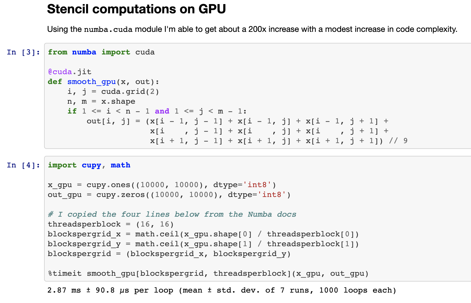
Enter [numba.cuda.jit](https://numba.pydata.org/numba-doc/dev/cuda/index.html)
Numba's backend for CUDA. Numba.cuda.jit allows Python users to author,
compile, and run CUDA code, written in Python, interactively without leaving a
Python session. Here is an image of writing a stencil computation that
smoothes a 2d-image all from within a Jupyter Notebook:
Here is a simplified comparison of Numba CPU/GPU code to compare programming
style..
The GPU code gets a 200x speed improvement over a single CPU core.
### CPU -- 600 ms
```python
@numba.jit
def _smooth(x):
out = np.empty_like(x)
for i in range(1, x.shape[0] - 1):
for j in range(1, x.shape[1] - 1):
out[i, j] = x[i + -1, j + -1] + x[i + -1, j + 0] + x[i + -1, j + 1] +
x[i + 0, j + -1] + x[i + 0, j + 0] + x[i + 0, j + 1] +
x[i + 1, j + -1] + x[i + 1, j + 0] + x[i + 1, j + 1]) // 9
return out
```
or if we use the fancy numba.stencil decorator ...
```python
@numba.stencil
def _smooth(x):
return (x[-1, -1] + x[-1, 0] + x[-1, 1] +
x[ 0, -1] + x[ 0, 0] + x[ 0, 1] +
x[ 1, -1] + x[ 1, 0] + x[ 1, 1]) // 9
```
### GPU -- 3 ms
```python
@numba.cuda.jit
def smooth_gpu(x, out):
i, j = cuda.grid(2)
n, m = x.shape
if 1 <= i < n - 1 and 1 <= j < m - 1:
out[i, j] = (x[i - 1, j - 1] + x[i - 1, j] + x[i - 1, j + 1] +
x[i , j - 1] + x[i , j] + x[i , j + 1] +
x[i + 1, j - 1] + x[i + 1, j] + x[i + 1, j + 1]) // 9
```
Numba.cuda.jit has been out in the wild for years.
It's accessible, mature, and fun to play with.
If you have a machine with a GPU in it and some curiosity
then we strongly recommend that you try it out.
```
conda install numba
# or
pip install numba
```
```python
>>> import numba.cuda
```
## Scaling with Dask
As mentioned in previous blogposts
(
[1](https://blog.dask.org/2019/01/03/dask-array-gpus-first-steps),
[2](https://blog.dask.org/2019/01/13/dask-cudf-first-steps),
[3](https://blog.dask.org/2019/03/04/building-gpu-groupbys),
[4](https://blog.dask.org/2019/03/18/dask-nep18)
)
we've been generalizing [Dask](https://dask.org), to operate not just with
Numpy arrays and Pandas dataframes, but with anything that looks enough like
Numpy (like [CuPy](https://cupy.chainer.org/) or
[Sparse](https://sparse.pydata.org/en/latest/) or
[Jax](https://github.com/google/jax)) or enough like Pandas (like [RAPIDS
cuDF](https://docs.rapids.ai/api/cudf/nightly/))
to scale those libraries out too. This is working out well. Here is a brief
video showing Dask array computing an SVD in parallel, and seeing what happens
when we swap out the Numpy library for CuPy.
We see that there is about a 10x speed improvement on the computation. Most
importantly, we were able to switch between a CPU implementation and a GPU
implementation with a small one-line change, but continue using the
sophisticated algorithms with Dask Array, like it's parallel SVD
implementation.
We also saw a relative slowdown in communication. In general almost all
non-trivial Dask + GPU work today is becoming communication-bound. We've
gotten fast enough at computation that the relative importance of communication
has grown significantly. We're working to resolve this with our next topic,
UCX.
## Communication with UCX
_See [this talk](https://developer.download.nvidia.com/video/gputechconf/gtc/2019/video/S9679/s9679-ucx-python-a-flexible-communication-library-for-python-applications.mp4) by [Akshay
Venkatesh](https://github.com/Akshay-Venkatesh) or view [the
slides](https://www.slideshare.net/MatthewRocklin/ucxpython-a-flexible-communication-library-for-python-applications)_
_Also see [this recent blogpost about UCX and
Dask](https://blog.dask.org/2019/06/09/ucx-dgx)_
We've been integrating the [OpenUCX](https://openucx.org) library into Python
with [UCX-Py](https://github.com/rapidsai/ucx-py). UCX provides uniform access
to transports like TCP, InfiniBand, shared memory, and NVLink. UCX-Py is the
first time that access to many of these transports has been easily accessible
from the Python language.
Using UCX and Dask together we're able to get significant speedups. Here is a
trace of the SVD computation from before both before and after adding UCX:
**Before UCX**:
**After UCX**:
There is still a great deal to do here though (the blogpost linked above has
several items in the Future Work section).
People can try out UCX and UCX-Py with highly experimental conda packages:
```
conda create -n ucx -c conda-forge -c jakirkham/label/ucx cudatoolkit=9.2 ucx-proc=*=gpu ucx ucx-py python=3.7
```
We hope that this work will also affect non-GPU users on HPC systems with
Infiniband, or even users on consumer hardware due to the easy access to shared
memory communication.
## Packaging
In an [earlier blogpost](https://matthewrocklin.com/blog/work/2018/12/17/gpu-python-challenges)
we discussed the challenges around installing the wrong versions of CUDA
enabled packages that don't match the CUDA driver installed on the system.
Fortunately due to recent work from [Stan Seibert](https://github.com/seibert)
and [Michael Sarahan](https://github.com/msarahan) at Anaconda, Conda 4.7 now
has a special `cuda` meta-package that is set to the version of the installed
driver. This should make it much easier for users in the future to install the
correct package.
Conda 4.7 was just releasead, and comes with many new features other than the
`cuda` meta-package. You can read more about it [here](https://www.anaconda.com/how-we-made-conda-faster-4-7/).
```
conda update conda
```
There is still plenty of work to do in the packaging space today.
Everyone who builds conda packages does it their own way,
resulting in headache and heterogeneity.
This is largely due to not having centralized infrastructure
to build and test CUDA enabled packages,
like we have in [Conda Forge](https://conda-forge.org).
Fortunately, the Conda Forge community is working together with Anaconda and
NVIDIA to help resolve this, though that will likely take some time.
## Summary
This post gave an update of the status of some of the efforts behind GPU
computing in Python. It also provided a variety of links for future reading.
We include them below if you would like to learn more:
- [Slides](https://docs.google.com/presentation/d/e/2PACX-1vSajAH6FzgQH4OwOJD5y-t9mjF9tTKEeljguEsfcjavp18pL4LkpABy4lW2uMykIUvP2dC-1AmhCq6l/pub?start=false&loop=false&delayms=60000)
- Numpy on the GPU: [CuPy](https://cupy.chainer.org/)
- Numpy on the GPU (again): [Jax](https://github.com/google/jax)
- Pandas on the GPU: [RAPIDS cuDF](https://docs.rapids.ai/api/cudf/nightly/)
- Scikit-Learn on the GPU: [RAPIDS cuML](https://docs.rapids.ai/api/cuml/nightly/)
- [Benchmark suite](https://github.com/pentschev/pybench)
- [Numba CUDA JIT notebook](https://gist.github.com/mrocklin/9272bf84a8faffdbbe2cd44b4bc4ce3c)
- [A talk on UCX](https://developer.download.nvidia.com/video/gputechconf/gtc/2019/video/S9679/s9679-ucx-python-a-flexible-communication-library-for-python-applications.mp4)
- [A blogpost on UCX and Dask](https://blog.dask.org/2019/06/09/ucx-dgx)
- [Conda 4.7](https://www.anaconda.com/how-we-made-conda-faster-4-7/)
 Here is a simplified comparison of Numba CPU/GPU code to compare programming
style..
The GPU code gets a 200x speed improvement over a single CPU core.
### CPU -- 600 ms
```python
@numba.jit
def _smooth(x):
out = np.empty_like(x)
for i in range(1, x.shape[0] - 1):
for j in range(1, x.shape[1] - 1):
out[i, j] = x[i + -1, j + -1] + x[i + -1, j + 0] + x[i + -1, j + 1] +
x[i + 0, j + -1] + x[i + 0, j + 0] + x[i + 0, j + 1] +
x[i + 1, j + -1] + x[i + 1, j + 0] + x[i + 1, j + 1]) // 9
return out
```
or if we use the fancy numba.stencil decorator ...
```python
@numba.stencil
def _smooth(x):
return (x[-1, -1] + x[-1, 0] + x[-1, 1] +
x[ 0, -1] + x[ 0, 0] + x[ 0, 1] +
x[ 1, -1] + x[ 1, 0] + x[ 1, 1]) // 9
```
### GPU -- 3 ms
```python
@numba.cuda.jit
def smooth_gpu(x, out):
i, j = cuda.grid(2)
n, m = x.shape
if 1 <= i < n - 1 and 1 <= j < m - 1:
out[i, j] = (x[i - 1, j - 1] + x[i - 1, j] + x[i - 1, j + 1] +
x[i , j - 1] + x[i , j] + x[i , j + 1] +
x[i + 1, j - 1] + x[i + 1, j] + x[i + 1, j + 1]) // 9
```
Numba.cuda.jit has been out in the wild for years.
It's accessible, mature, and fun to play with.
If you have a machine with a GPU in it and some curiosity
then we strongly recommend that you try it out.
```
conda install numba
# or
pip install numba
```
```python
>>> import numba.cuda
```
## Scaling with Dask
As mentioned in previous blogposts
(
[1](https://blog.dask.org/2019/01/03/dask-array-gpus-first-steps),
[2](https://blog.dask.org/2019/01/13/dask-cudf-first-steps),
[3](https://blog.dask.org/2019/03/04/building-gpu-groupbys),
[4](https://blog.dask.org/2019/03/18/dask-nep18)
)
we've been generalizing [Dask](https://dask.org), to operate not just with
Numpy arrays and Pandas dataframes, but with anything that looks enough like
Numpy (like [CuPy](https://cupy.chainer.org/) or
[Sparse](https://sparse.pydata.org/en/latest/) or
[Jax](https://github.com/google/jax)) or enough like Pandas (like [RAPIDS
cuDF](https://docs.rapids.ai/api/cudf/nightly/))
to scale those libraries out too. This is working out well. Here is a brief
video showing Dask array computing an SVD in parallel, and seeing what happens
when we swap out the Numpy library for CuPy.
We see that there is about a 10x speed improvement on the computation. Most
importantly, we were able to switch between a CPU implementation and a GPU
implementation with a small one-line change, but continue using the
sophisticated algorithms with Dask Array, like it's parallel SVD
implementation.
We also saw a relative slowdown in communication. In general almost all
non-trivial Dask + GPU work today is becoming communication-bound. We've
gotten fast enough at computation that the relative importance of communication
has grown significantly. We're working to resolve this with our next topic,
UCX.
## Communication with UCX
_See [this talk](https://developer.download.nvidia.com/video/gputechconf/gtc/2019/video/S9679/s9679-ucx-python-a-flexible-communication-library-for-python-applications.mp4) by [Akshay
Venkatesh](https://github.com/Akshay-Venkatesh) or view [the
slides](https://www.slideshare.net/MatthewRocklin/ucxpython-a-flexible-communication-library-for-python-applications)_
_Also see [this recent blogpost about UCX and
Dask](https://blog.dask.org/2019/06/09/ucx-dgx)_
We've been integrating the [OpenUCX](https://openucx.org) library into Python
with [UCX-Py](https://github.com/rapidsai/ucx-py). UCX provides uniform access
to transports like TCP, InfiniBand, shared memory, and NVLink. UCX-Py is the
first time that access to many of these transports has been easily accessible
from the Python language.
Using UCX and Dask together we're able to get significant speedups. Here is a
trace of the SVD computation from before both before and after adding UCX:
**Before UCX**:
**After UCX**:
There is still a great deal to do here though (the blogpost linked above has
several items in the Future Work section).
People can try out UCX and UCX-Py with highly experimental conda packages:
```
conda create -n ucx -c conda-forge -c jakirkham/label/ucx cudatoolkit=9.2 ucx-proc=*=gpu ucx ucx-py python=3.7
```
We hope that this work will also affect non-GPU users on HPC systems with
Infiniband, or even users on consumer hardware due to the easy access to shared
memory communication.
## Packaging
In an [earlier blogpost](https://matthewrocklin.com/blog/work/2018/12/17/gpu-python-challenges)
we discussed the challenges around installing the wrong versions of CUDA
enabled packages that don't match the CUDA driver installed on the system.
Fortunately due to recent work from [Stan Seibert](https://github.com/seibert)
and [Michael Sarahan](https://github.com/msarahan) at Anaconda, Conda 4.7 now
has a special `cuda` meta-package that is set to the version of the installed
driver. This should make it much easier for users in the future to install the
correct package.
Conda 4.7 was just releasead, and comes with many new features other than the
`cuda` meta-package. You can read more about it [here](https://www.anaconda.com/how-we-made-conda-faster-4-7/).
```
conda update conda
```
There is still plenty of work to do in the packaging space today.
Everyone who builds conda packages does it their own way,
resulting in headache and heterogeneity.
This is largely due to not having centralized infrastructure
to build and test CUDA enabled packages,
like we have in [Conda Forge](https://conda-forge.org).
Fortunately, the Conda Forge community is working together with Anaconda and
NVIDIA to help resolve this, though that will likely take some time.
## Summary
This post gave an update of the status of some of the efforts behind GPU
computing in Python. It also provided a variety of links for future reading.
We include them below if you would like to learn more:
- [Slides](https://docs.google.com/presentation/d/e/2PACX-1vSajAH6FzgQH4OwOJD5y-t9mjF9tTKEeljguEsfcjavp18pL4LkpABy4lW2uMykIUvP2dC-1AmhCq6l/pub?start=false&loop=false&delayms=60000)
- Numpy on the GPU: [CuPy](https://cupy.chainer.org/)
- Numpy on the GPU (again): [Jax](https://github.com/google/jax)
- Pandas on the GPU: [RAPIDS cuDF](https://docs.rapids.ai/api/cudf/nightly/)
- Scikit-Learn on the GPU: [RAPIDS cuML](https://docs.rapids.ai/api/cuml/nightly/)
- [Benchmark suite](https://github.com/pentschev/pybench)
- [Numba CUDA JIT notebook](https://gist.github.com/mrocklin/9272bf84a8faffdbbe2cd44b4bc4ce3c)
- [A talk on UCX](https://developer.download.nvidia.com/video/gputechconf/gtc/2019/video/S9679/s9679-ucx-python-a-flexible-communication-library-for-python-applications.mp4)
- [A blogpost on UCX and Dask](https://blog.dask.org/2019/06/09/ucx-dgx)
- [Conda 4.7](https://www.anaconda.com/how-we-made-conda-faster-4-7/)
Here is a simplified comparison of Numba CPU/GPU code to compare programming
style..
The GPU code gets a 200x speed improvement over a single CPU core.
### CPU -- 600 ms
```python
@numba.jit
def _smooth(x):
out = np.empty_like(x)
for i in range(1, x.shape[0] - 1):
for j in range(1, x.shape[1] - 1):
out[i, j] = x[i + -1, j + -1] + x[i + -1, j + 0] + x[i + -1, j + 1] +
x[i + 0, j + -1] + x[i + 0, j + 0] + x[i + 0, j + 1] +
x[i + 1, j + -1] + x[i + 1, j + 0] + x[i + 1, j + 1]) // 9
return out
```
or if we use the fancy numba.stencil decorator ...
```python
@numba.stencil
def _smooth(x):
return (x[-1, -1] + x[-1, 0] + x[-1, 1] +
x[ 0, -1] + x[ 0, 0] + x[ 0, 1] +
x[ 1, -1] + x[ 1, 0] + x[ 1, 1]) // 9
```
### GPU -- 3 ms
```python
@numba.cuda.jit
def smooth_gpu(x, out):
i, j = cuda.grid(2)
n, m = x.shape
if 1 <= i < n - 1 and 1 <= j < m - 1:
out[i, j] = (x[i - 1, j - 1] + x[i - 1, j] + x[i - 1, j + 1] +
x[i , j - 1] + x[i , j] + x[i , j + 1] +
x[i + 1, j - 1] + x[i + 1, j] + x[i + 1, j + 1]) // 9
```
Numba.cuda.jit has been out in the wild for years.
It's accessible, mature, and fun to play with.
If you have a machine with a GPU in it and some curiosity
then we strongly recommend that you try it out.
```
conda install numba
# or
pip install numba
```
```python
>>> import numba.cuda
```
## Scaling with Dask
As mentioned in previous blogposts
(
[1](https://blog.dask.org/2019/01/03/dask-array-gpus-first-steps),
[2](https://blog.dask.org/2019/01/13/dask-cudf-first-steps),
[3](https://blog.dask.org/2019/03/04/building-gpu-groupbys),
[4](https://blog.dask.org/2019/03/18/dask-nep18)
)
we've been generalizing [Dask](https://dask.org), to operate not just with
Numpy arrays and Pandas dataframes, but with anything that looks enough like
Numpy (like [CuPy](https://cupy.chainer.org/) or
[Sparse](https://sparse.pydata.org/en/latest/) or
[Jax](https://github.com/google/jax)) or enough like Pandas (like [RAPIDS
cuDF](https://docs.rapids.ai/api/cudf/nightly/))
to scale those libraries out too. This is working out well. Here is a brief
video showing Dask array computing an SVD in parallel, and seeing what happens
when we swap out the Numpy library for CuPy.
We see that there is about a 10x speed improvement on the computation. Most
importantly, we were able to switch between a CPU implementation and a GPU
implementation with a small one-line change, but continue using the
sophisticated algorithms with Dask Array, like it's parallel SVD
implementation.
We also saw a relative slowdown in communication. In general almost all
non-trivial Dask + GPU work today is becoming communication-bound. We've
gotten fast enough at computation that the relative importance of communication
has grown significantly. We're working to resolve this with our next topic,
UCX.
## Communication with UCX
_See [this talk](https://developer.download.nvidia.com/video/gputechconf/gtc/2019/video/S9679/s9679-ucx-python-a-flexible-communication-library-for-python-applications.mp4) by [Akshay
Venkatesh](https://github.com/Akshay-Venkatesh) or view [the
slides](https://www.slideshare.net/MatthewRocklin/ucxpython-a-flexible-communication-library-for-python-applications)_
_Also see [this recent blogpost about UCX and
Dask](https://blog.dask.org/2019/06/09/ucx-dgx)_
We've been integrating the [OpenUCX](https://openucx.org) library into Python
with [UCX-Py](https://github.com/rapidsai/ucx-py). UCX provides uniform access
to transports like TCP, InfiniBand, shared memory, and NVLink. UCX-Py is the
first time that access to many of these transports has been easily accessible
from the Python language.
Using UCX and Dask together we're able to get significant speedups. Here is a
trace of the SVD computation from before both before and after adding UCX:
**Before UCX**:
**After UCX**:
There is still a great deal to do here though (the blogpost linked above has
several items in the Future Work section).
People can try out UCX and UCX-Py with highly experimental conda packages:
```
conda create -n ucx -c conda-forge -c jakirkham/label/ucx cudatoolkit=9.2 ucx-proc=*=gpu ucx ucx-py python=3.7
```
We hope that this work will also affect non-GPU users on HPC systems with
Infiniband, or even users on consumer hardware due to the easy access to shared
memory communication.
## Packaging
In an [earlier blogpost](https://matthewrocklin.com/blog/work/2018/12/17/gpu-python-challenges)
we discussed the challenges around installing the wrong versions of CUDA
enabled packages that don't match the CUDA driver installed on the system.
Fortunately due to recent work from [Stan Seibert](https://github.com/seibert)
and [Michael Sarahan](https://github.com/msarahan) at Anaconda, Conda 4.7 now
has a special `cuda` meta-package that is set to the version of the installed
driver. This should make it much easier for users in the future to install the
correct package.
Conda 4.7 was just releasead, and comes with many new features other than the
`cuda` meta-package. You can read more about it [here](https://www.anaconda.com/how-we-made-conda-faster-4-7/).
```
conda update conda
```
There is still plenty of work to do in the packaging space today.
Everyone who builds conda packages does it their own way,
resulting in headache and heterogeneity.
This is largely due to not having centralized infrastructure
to build and test CUDA enabled packages,
like we have in [Conda Forge](https://conda-forge.org).
Fortunately, the Conda Forge community is working together with Anaconda and
NVIDIA to help resolve this, though that will likely take some time.
## Summary
This post gave an update of the status of some of the efforts behind GPU
computing in Python. It also provided a variety of links for future reading.
We include them below if you would like to learn more:
- [Slides](https://docs.google.com/presentation/d/e/2PACX-1vSajAH6FzgQH4OwOJD5y-t9mjF9tTKEeljguEsfcjavp18pL4LkpABy4lW2uMykIUvP2dC-1AmhCq6l/pub?start=false&loop=false&delayms=60000)
- Numpy on the GPU: [CuPy](https://cupy.chainer.org/)
- Numpy on the GPU (again): [Jax](https://github.com/google/jax)
- Pandas on the GPU: [RAPIDS cuDF](https://docs.rapids.ai/api/cudf/nightly/)
- Scikit-Learn on the GPU: [RAPIDS cuML](https://docs.rapids.ai/api/cuml/nightly/)
- [Benchmark suite](https://github.com/pentschev/pybench)
- [Numba CUDA JIT notebook](https://gist.github.com/mrocklin/9272bf84a8faffdbbe2cd44b4bc4ce3c)
- [A talk on UCX](https://developer.download.nvidia.com/video/gputechconf/gtc/2019/video/S9679/s9679-ucx-python-a-flexible-communication-library-for-python-applications.mp4)
- [A blogpost on UCX and Dask](https://blog.dask.org/2019/06/09/ucx-dgx)
- [Conda 4.7](https://www.anaconda.com/how-we-made-conda-faster-4-7/)