---
blogpost: true
date: Aug 7, 2018
title: Building SAGA optimization for Dask arrays
tags: Programming, Python, scipy, dask
---
_This work is supported by [ETH Zurich](https://www.ethz.ch/en.html), [Anaconda
Inc](http://anaconda.com), and the [Berkeley Institute for Data
Science](https://bids.berkeley.edu/)_
At a recent Scikit-learn/Scikit-image/Dask sprint at BIDS, [Fabian Pedregosa](http://fa.bianp.net) (a
machine learning researcher and Scikit-learn developer) and Matthew
Rocklin (Dask core developer) sat down together to develop an implementation of the incremental optimization algorithm
[SAGA](https://arxiv.org/pdf/1407.0202.pdf) on parallel Dask datasets. The result is a sequential algorithm that can be run on any dask array, and so allows the data to be stored on disk or even distributed among different machines.
It was interesting both to see how the algorithm performed and also to see
the ease and challenges to run a research algorithm on a Dask distributed dataset.
### Start
We started with an initial implementation that Fabian had written for Numpy
arrays using Numba. The following code solves an optimization problem of the form
$$
min_x \sum_{i=1}^n f(a_i^t x, b_i)
$$
```python
import numpy as np
from numba import njit
from sklearn.linear_model.sag import get_auto_step_size
from sklearn.utils.extmath import row_norms
@njit
def deriv_logistic(p, y):
# derivative of logistic loss
# same as in lightning (with minus sign)
p *= y
if p > 0:
phi = 1. / (1 + np.exp(-p))
else:
exp_t = np.exp(p)
phi = exp_t / (1. + exp_t)
return (phi - 1) * y
@njit
def SAGA(A, b, step_size, max_iter=100):
"""
SAGA algorithm
A : n_samples x n_features numpy array
b : n_samples numpy array with values -1 or 1
"""
n_samples, n_features = A.shape
memory_gradient = np.zeros(n_samples)
gradient_average = np.zeros(n_features)
x = np.zeros(n_features) # vector of coefficients
step_size = 0.3 * get_auto_step_size(row_norms(A, squared=True).max(), 0, 'log', False)
for _ in range(max_iter):
# sample randomly
idx = np.arange(memory_gradient.size)
np.random.shuffle(idx)
# .. inner iteration ..
for i in idx:
grad_i = deriv_logistic(np.dot(x, A[i]), b[i])
# .. update coefficients ..
delta = (grad_i - memory_gradient[i]) * A[i]
x -= step_size * (delta + gradient_average)
# .. update memory terms ..
gradient_average += (grad_i - memory_gradient[i]) * A[i] / n_samples
memory_gradient[i] = grad_i
# monitor convergence
print('gradient norm:', np.linalg.norm(gradient_average))
return x
```
This implementation is a simplified version of the [SAGA
implementation](https://github.com/openopt/copt/blob/master/copt/randomized.py)
that Fabian uses regularly as part of his research, and that assumes that $f$ is the [logistic loss](https://en.wikipedia.org/wiki/Loss_functions_for_classification#Logistic_loss), i.e., $f(z) = \log(1 + \exp(-z))$. It can be used to solve problems with other values of $f$ by overwriting the function deriv_logistic.
We wanted to apply it across a parallel Dask array by applying it to each chunk of the Dask array, a smaller Numpy array, one at a time, carrying along a set of parameters along the way.
### Development Process
In order to better understand the challenges of writing Dask algorithms, Fabian
did most of the actual coding to start. Fabian is good example of a researcher who
knows how to program well and how to design ML algorithms, but has no direct
exposure to the Dask library. This was an educational opportunity both for
Fabian and for Matt. Fabian learned how to use Dask, and Matt learned how to
introduce Dask to researchers like Fabian.
### Step 1: Build a sequential algorithm with pure functions
To start we actually didn't use Dask at all, instead, Fabian modified his implementation in a few ways:
1. It should operate over a list of Numpy arrays. A list of Numpy arrays is similar to a Dask array, but simpler.
2. It should separate blocks of logic into separate functions, these will
eventually become tasks, so they should be sizable chunks of work. In this
case, this led to the creating of the function `_chunk_saga` that
performs an iteration of the SAGA algorithm on a subset of the data.
3. These functions should not modify their inputs, nor should they depend on
global state. All information that those functions require (like
the parameters that we're learning in our algorithm) should be
explicitly provided as inputs.
These requested modifications affect performance a bit, we end up making more
copies of the parameters and more copies of intermediate state. In terms of
programming difficulty this took a bit of time (around a couple hours) but is a
straightforward task that Fabian didn't seem to find challenging or foreign.
These changes resulted in the following code:
```python
from numba import njit
from sklearn.utils.extmath import row_norms
from sklearn.linear_model.sag import get_auto_step_size
@njit
def _chunk_saga(A, b, n_samples, f_deriv, x, memory_gradient, gradient_average, step_size):
# Make explicit copies of inputs
x = x.copy()
gradient_average = gradient_average.copy()
memory_gradient = memory_gradient.copy()
# Sample randomly
idx = np.arange(memory_gradient.size)
np.random.shuffle(idx)
# .. inner iteration ..
for i in idx:
grad_i = f_deriv(np.dot(x, A[i]), b[i])
# .. update coefficients ..
delta = (grad_i - memory_gradient[i]) * A[i]
x -= step_size * (delta + gradient_average)
# .. update memory terms ..
gradient_average += (grad_i - memory_gradient[i]) * A[i] / n_samples
memory_gradient[i] = grad_i
return x, memory_gradient, gradient_average
def full_saga(data, max_iter=100, callback=None):
"""
data: list of (A, b), where A is a n_samples x n_features
numpy array and b is a n_samples numpy array
"""
n_samples = 0
for A, b in data:
n_samples += A.shape[0]
n_features = data[0][0].shape[1]
memory_gradients = [np.zeros(A.shape[0]) for (A, b) in data]
gradient_average = np.zeros(n_features)
x = np.zeros(n_features)
steps = [get_auto_step_size(row_norms(A, squared=True).max(), 0, 'log', False) for (A, b) in data]
step_size = 0.3 * np.min(steps)
for _ in range(max_iter):
for i, (A, b) in enumerate(data):
x, memory_gradients[i], gradient_average = _chunk_saga(
A, b, n_samples, deriv_logistic, x, memory_gradients[i],
gradient_average, step_size)
if callback is not None:
print(callback(x, data))
return x
```
### Step 2: Apply dask.delayed
Once functions neither modified their inputs nor relied on global state we went
over a [dask.delayed example](https://mybinder.org/v2/gh/dask/dask-examples/main?urlpath=%2Ftree%2Fdelayed.ipynb),
and then applied the `@dask.delayed` decorator to the functions that
Fabian had written. Fabian did this at first in about five minutes and to our
mutual surprise, things actually worked
```python
@dask.delayed(nout=3) # <<<---- New
@njit
def _chunk_saga(A, b, n_samples, f_deriv, x, memory_gradient, gradient_average, step_size):
...
def full_saga(data, max_iter=100, callback=None):
n_samples = 0
for A, b in data:
n_samples += A.shape[0]
data = dask.persist(*data) # <<<---- New
...
for _ in range(max_iter):
for i, (A, b) in enumerate(data):
x, memory_gradients[i], gradient_average = _chunk_saga(
A, b, n_samples, deriv_logistic, x, memory_gradients[i],
gradient_average, step_size)
cb = dask.delayed(callback)(x, data) # <<<---- Changed
x, cb = dask.persist(x, cb) # <<<---- New
print(cb.compute()
```
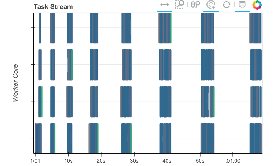
However, they didn't work _that well_. When we took a look at the dask
dashboard we find that there is a lot of dead space, a sign that we're still
doing a lot of computation on the client side.
 ### Step 3: Diagnose and add more dask.delayed calls
While things worked, they were also fairly slow. If you notice the
dashboard plot above you'll see that there is plenty of white in between
colored rectangles. This shows that there are long periods where none of the
workers is doing any work.
This is a common sign that we're mixing work between the workers (which shows
up on the dashbaord) and the client. The solution to this is usually more
targetted use of dask.delayed. Dask delayed is trivial to start using, but
does require some experience to use well. It's important to keep track of
which operations and variables are delayed and which aren't. There is some
cost to mixing between them.
At this point Matt stepped in and added delayed in a few more places and the
dashboard plot started looking cleaner.
```python
@dask.delayed(nout=3) # <<<---- New
@njit
def _chunk_saga(A, b, n_samples, f_deriv, x, memory_gradient, gradient_average, step_size):
...
def full_saga(data, max_iter=100, callback=None):
n_samples = 0
for A, b in data:
n_samples += A.shape[0]
n_features = data[0][0].shape[1]
data = dask.persist(*data) # <<<---- New
memory_gradients = [dask.delayed(np.zeros)(A.shape[0])
for (A, b) in data] # <<<---- Changed
gradient_average = dask.delayed(np.zeros)(n_features) # Changed
x = dask.delayed(np.zeros)(n_features) # <<<---- Changed
steps = [dask.delayed(get_auto_step_size)(
dask.delayed(row_norms)(A, squared=True).max(),
0, 'log', False)
for (A, b) in data] # <<<---- Changed
step_size = 0.3 * dask.delayed(np.min)(steps) # <<<---- Changed
for _ in range(max_iter):
for i, (A, b) in enumerate(data):
x, memory_gradients[i], gradient_average = _chunk_saga(
A, b, n_samples, deriv_logistic, x, memory_gradients[i],
gradient_average, step_size)
cb = dask.delayed(callback)(x, data) # <<<---- Changed
x, memory_gradients, gradient_average, step_size, cb = \
dask.persist(x, memory_gradients, gradient_average, step_size, cb) # New
print(cb.compute()) # <<<---- changed
return x
```
### Step 3: Diagnose and add more dask.delayed calls
While things worked, they were also fairly slow. If you notice the
dashboard plot above you'll see that there is plenty of white in between
colored rectangles. This shows that there are long periods where none of the
workers is doing any work.
This is a common sign that we're mixing work between the workers (which shows
up on the dashbaord) and the client. The solution to this is usually more
targetted use of dask.delayed. Dask delayed is trivial to start using, but
does require some experience to use well. It's important to keep track of
which operations and variables are delayed and which aren't. There is some
cost to mixing between them.
At this point Matt stepped in and added delayed in a few more places and the
dashboard plot started looking cleaner.
```python
@dask.delayed(nout=3) # <<<---- New
@njit
def _chunk_saga(A, b, n_samples, f_deriv, x, memory_gradient, gradient_average, step_size):
...
def full_saga(data, max_iter=100, callback=None):
n_samples = 0
for A, b in data:
n_samples += A.shape[0]
n_features = data[0][0].shape[1]
data = dask.persist(*data) # <<<---- New
memory_gradients = [dask.delayed(np.zeros)(A.shape[0])
for (A, b) in data] # <<<---- Changed
gradient_average = dask.delayed(np.zeros)(n_features) # Changed
x = dask.delayed(np.zeros)(n_features) # <<<---- Changed
steps = [dask.delayed(get_auto_step_size)(
dask.delayed(row_norms)(A, squared=True).max(),
0, 'log', False)
for (A, b) in data] # <<<---- Changed
step_size = 0.3 * dask.delayed(np.min)(steps) # <<<---- Changed
for _ in range(max_iter):
for i, (A, b) in enumerate(data):
x, memory_gradients[i], gradient_average = _chunk_saga(
A, b, n_samples, deriv_logistic, x, memory_gradients[i],
gradient_average, step_size)
cb = dask.delayed(callback)(x, data) # <<<---- Changed
x, memory_gradients, gradient_average, step_size, cb = \
dask.persist(x, memory_gradients, gradient_average, step_size, cb) # New
print(cb.compute()) # <<<---- changed
return x
```
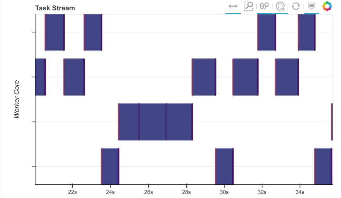 From a dask perspective this now looks good. We see that one `partial_fit`
call is active at any given time with no large horizontal gaps between
`partial_fit` calls. We're not getting any parallelism (this is just a
sequential algorithm) but we don't have much dead space. The model seems to
jump between the various workers, processing on a chunk of data before moving
on to new data.
### Step 4: Profile
The dashboard image above gives confidence that our algorithm is operating as
it should. The block-sequential nature of the algorithm comes out cleanly, and
the gaps between tasks are very short.
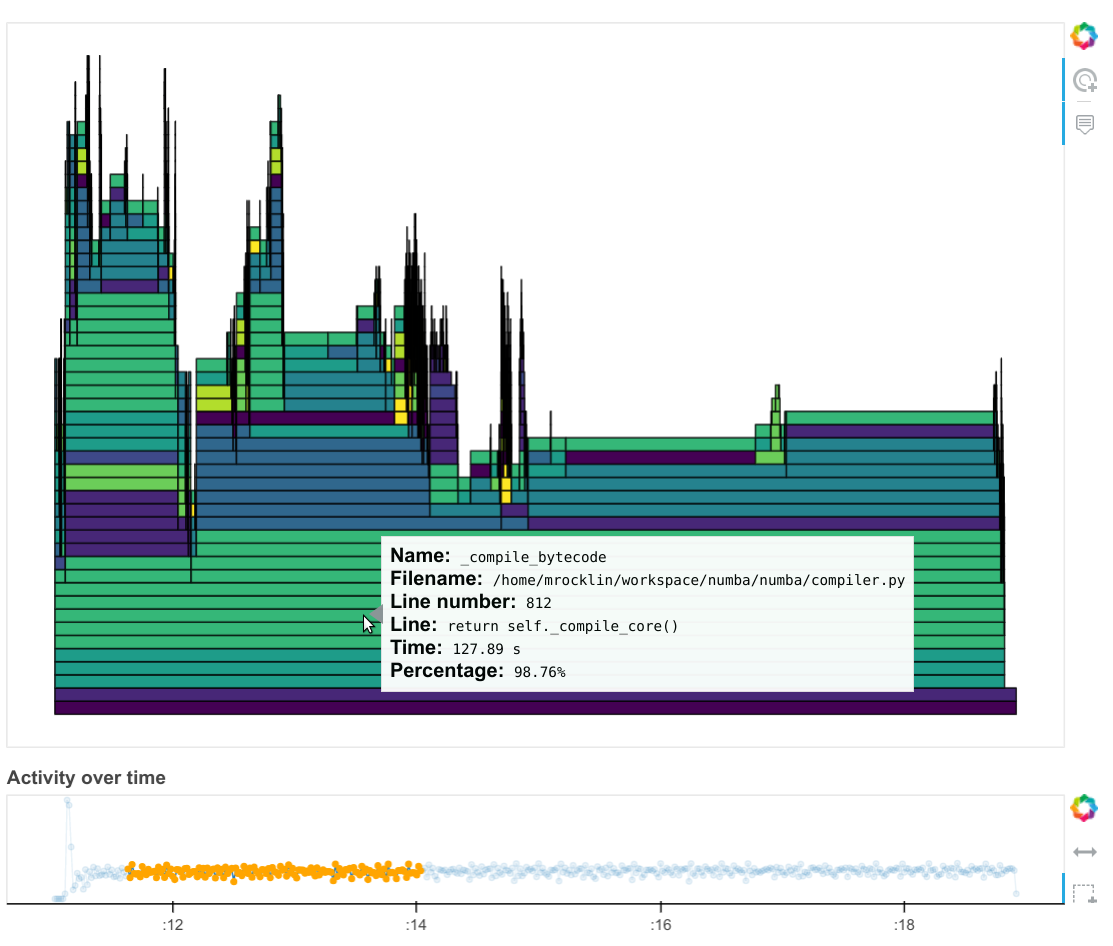
However, when we look at the profile plot of the computation across all of our
cores (Dask constantly runs a profiler on all threads on all workers to get
this information) we see that most of our time is spent compiling Numba code.
From a dask perspective this now looks good. We see that one `partial_fit`
call is active at any given time with no large horizontal gaps between
`partial_fit` calls. We're not getting any parallelism (this is just a
sequential algorithm) but we don't have much dead space. The model seems to
jump between the various workers, processing on a chunk of data before moving
on to new data.
### Step 4: Profile
The dashboard image above gives confidence that our algorithm is operating as
it should. The block-sequential nature of the algorithm comes out cleanly, and
the gaps between tasks are very short.
However, when we look at the profile plot of the computation across all of our
cores (Dask constantly runs a profiler on all threads on all workers to get
this information) we see that most of our time is spent compiling Numba code.
 We started a conversation for this on the [numba issue
tracker](https://github.com/numba/numba/issues/3026) which has since been
resolved. That same computation over the same time now looks like this:
We started a conversation for this on the [numba issue
tracker](https://github.com/numba/numba/issues/3026) which has since been
resolved. That same computation over the same time now looks like this:
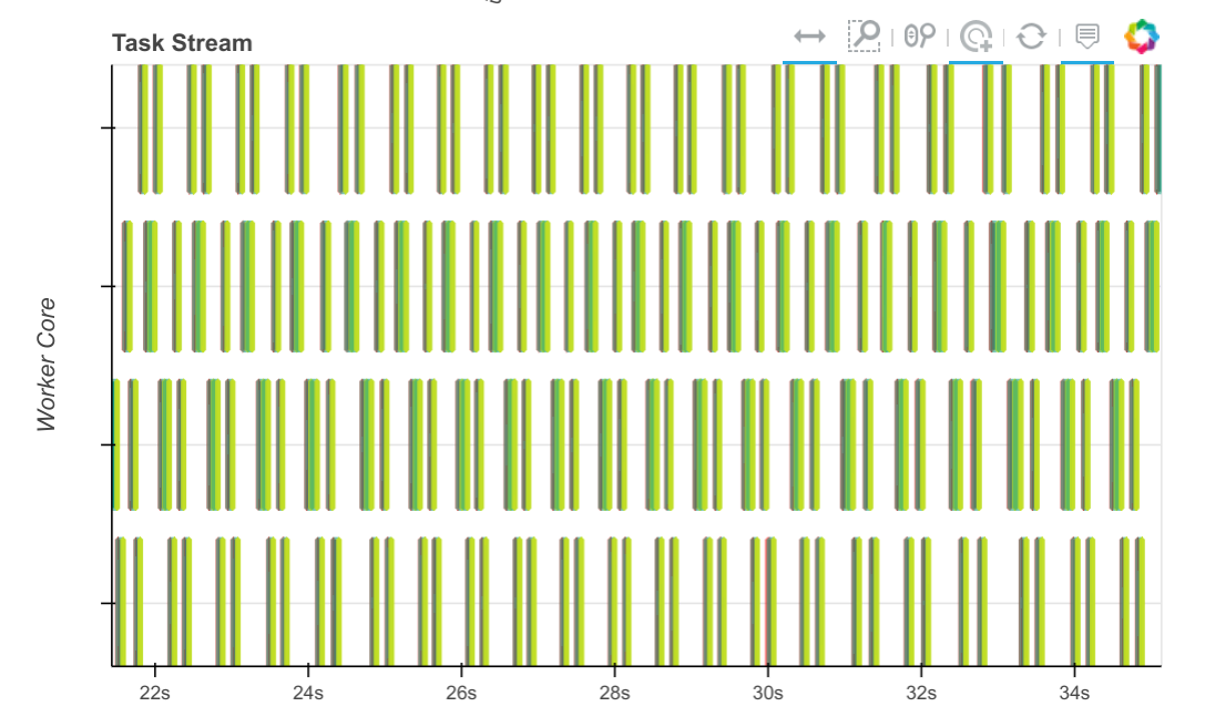 The tasks, which used to take seconds, now take tens of milliseconds, so we can
process through many more chunks in the same amount of time.
### Future Work
This was a useful experience to build an interesting algorithm. Most of the
work above took place in an afternoon. We came away from this activity
with a few tasks of our own:
1. Build a normal Scikit-Learn style estimator class for this algorithm
so that people can use it without thinking too much about delayed objects,
and can instead just use dask arrays or dataframes
2. Integrate some of Fabian's research on this algorithm that improves performance with
[sparse data and in multi-threaded environments](https://arxiv.org/pdf/1707.06468.pdf).
3. Think about how to improve the learning experience so that dask.delayed can
teach new users how to use it correctly
### Links
- [Notebooks for different stages of SAGA+Dask implementation](https://gist.github.com/5282dcf47505e2a1d214fd15c7da0ec3)
- [Scikit-Learn/Image + Dask Sprint issue tracker](https://github.com/scisprints/2018_05_sklearn_skimage_dask)
- [Paper on SAGA algorithm](https://github.com/scisprints/2018_05_sklearn_skimage_dask)
- [Fabian's more fully featured non-Dask SAGA implementation](https://github.com/openopt/copt/blob/master/copt/randomized.py)
- [Numba issue on repeated deserialization](https://github.com/numba/numba/issues/3026)
The tasks, which used to take seconds, now take tens of milliseconds, so we can
process through many more chunks in the same amount of time.
### Future Work
This was a useful experience to build an interesting algorithm. Most of the
work above took place in an afternoon. We came away from this activity
with a few tasks of our own:
1. Build a normal Scikit-Learn style estimator class for this algorithm
so that people can use it without thinking too much about delayed objects,
and can instead just use dask arrays or dataframes
2. Integrate some of Fabian's research on this algorithm that improves performance with
[sparse data and in multi-threaded environments](https://arxiv.org/pdf/1707.06468.pdf).
3. Think about how to improve the learning experience so that dask.delayed can
teach new users how to use it correctly
### Links
- [Notebooks for different stages of SAGA+Dask implementation](https://gist.github.com/5282dcf47505e2a1d214fd15c7da0ec3)
- [Scikit-Learn/Image + Dask Sprint issue tracker](https://github.com/scisprints/2018_05_sklearn_skimage_dask)
- [Paper on SAGA algorithm](https://github.com/scisprints/2018_05_sklearn_skimage_dask)
- [Fabian's more fully featured non-Dask SAGA implementation](https://github.com/openopt/copt/blob/master/copt/randomized.py)
- [Numba issue on repeated deserialization](https://github.com/numba/numba/issues/3026)