---
blogpost: true
date: Apr 19, 2017
title: Asynchronous Optimization Algorithms with Dask
tags: Programming, Python, scipy
description: Computations that evolve on partial results
---
_This work is supported by [Continuum Analytics](http://continuum.io),
the [XDATA Program](http://www.darpa.mil/program/XDATA),
and the Data Driven Discovery Initiative from the [Moore
Foundation](https://www.moore.org/)._
## Summary
In a previous post [we built convex optimization algorithms with
Dask](/2017/03/22/dask-glm-1) that ran
efficiently on a distributed cluster and were important for a broad class of
statistical and machine learning algorithms.
We now extend that work by looking at _asynchronous algorithms_. We show the
following:
1. APIs within Dask to build asynchronous computations generally, not just for
machine learning and optimization
2. Reasons why asynchronous algorithms are valuable in machine learning
3. A concrete asynchronous algorithm (Async ADMM) and its performance on a
toy dataset
This blogpost is co-authored by [Chris White](https://github.com/moody-marlin/)
(Capital One) who knows optimization and [Matthew
Rocklin](http://matthewrocklin.com/) (Continuum Analytics) who knows
distributed computing.
[Reproducible notebook available here](https://gist.github.com/4fc08482f33d60cc90cc3f8723146de5)
## Asynchronous vs Blocking Algorithms
When we say _asynchronous_ we contrast it against synchronous or blocking.
In a blocking algorithm you send out a bunch of work and then wait for the
result. Dask's normal `.compute()` interface is blocking. Consider the
following computation where we score a bunch of inputs in parallel and then
find the best:
```python
import dask
scores = [dask.delayed(score)(x) for x in L] # many lazy calls to the score function
best = dask.delayed(max)(scores)
best = best.compute() # Trigger all computation and wait until complete
```
This _blocks_. We can't do anything while it runs. If we're in a Jupyter
notebook we'll see a little asterisk telling us that we have to wait.
 In a non-blocking or asynchronous algorithm we send out work and track results
as they come in. We are still able to run commands locally while our
computations run in the background (or on other computers in the cluster).
Dask has a variety of asynchronous APIs, but the simplest is probably the
[concurrent.futures](https://docs.python.org/3/library/concurrent.futures.html)
API where we submit functions and then can wait and act on their return.
```python
from dask.distributed import Client, as_completed
client = Client('scheduler-address:8786')
# Send out several computations
futures = [client.submit(score, x) for x in L]
# Find max as results arrive
best = 0
for future in as_completed(futures):
score = future.result()
if score > best:
best = score
```
These two solutions are computationally equivalent. They do the same work and
run in the same amount of time. The blocking `dask.delayed` solution is
probably simpler to write down but the non-blocking `futures + as_completed`
solution lets us be more _flexible_.
For example, if we get a score that is _good enough_ then we might stop early.
If we find that certain kinds of values are giving better scores than others
then we might submit more computations around those values while cancelling
others, changing our computation during execution.
This ability to monitor and adapt a computation during execution is one reason
why people choose asynchronous algorithms. In the case of optimization
algorithms we are doing a search process and frequently updating parameters.
If we are able to update those parameters more frequently then we may be able
to slightly improve every subsequently launched computation. Asynchronous
algorithms enable increased flow of information around the cluster in
comparison to more lock-step batch-iterative algorithms.
## Asynchronous ADMM
In our [last blogpost](/2017/03/22/dask-glm-1)
we showed a simplified implementation of [Alternating Direction Method of
Multipliers](http://stanford.edu/~boyd/admm.html) (ADMM) with
[dask.delayed](http://dask.pydata.org/en/latest/delayed.html). We saw that in
a distributed context it performed well when compared to a more traditional
distributed gradient descent. This algorithm works by solving a small
optimization problem on every chunk of our data using our current parameter
estimates, bringing these back to the local process, combining them, and then
sending out new computation on updated parameters.
Now we alter this algorithm to update asynchronously, so that our parameters
change continuously as partial results come in in real-time. Instead of
sending out and waiting on batches of results, we now consume and emit a
constant stream of tasks with slightly improved parameter estimates.
We show three algorithms in sequence:
1. Synchronous: The original synchronous algorithm
2. Asynchronous-single: updates parameters with every new result
3. Asynchronous-batched: updates with all results that have come in since we
last updated.
## Setup
We create fake data
```python
n, k, chunksize = 50000000, 100, 50000
beta = np.random.random(k) # random beta coefficients, no intercept
zero_idx = np.random.choice(len(beta), size=10)
beta[zero_idx] = 0 # set some parameters to 0
X = da.random.normal(0, 1, size=(n, k), chunks=(chunksize, k))
y = X.dot(beta) + da.random.normal(0, 2, size=n, chunks=(chunksize,)) # add noise
X, y = persist(X, y) # trigger computation in the background
```
We define local functions for ADMM. These correspond to solving an l1-regularized Linear
regression problem:
```python
def local_f(beta, X, y, z, u, rho):
return ((y - X.dot(beta)) **2).sum() + (rho / 2) * np.dot(beta - z + u,
beta - z + u)
def local_grad(beta, X, y, z, u, rho):
return 2 * X.T.dot(X.dot(beta) - y) + rho * (beta - z + u)
def shrinkage(beta, t):
return np.maximum(0, beta - t) - np.maximum(0, -beta - t)
local_update2 = partial(local_update, f=local_f, fprime=local_grad)
lamduh = 7.2 # regularization parameter
# algorithm parameters
rho = 1.2
abstol = 1e-4
reltol = 1e-2
z = np.zeros(p) # the initial consensus estimate
# an array of the individual "dual variables" and parameter estimates,
# one for each chunk of data
u = np.array([np.zeros(p) for i in range(nchunks)])
betas = np.array([np.zeros(p) for i in range(nchunks)])
```
Finally because ADMM doesn't want to work on distributed arrays, but instead
on lists of remote numpy arrays (one numpy array per chunk of the dask.array)
we convert each our Dask.arrays into a list of dask.delayed objects:
```python
XD = X.to_delayed().flatten().tolist() # a list of numpy arrays, one for each chunk
yD = y.to_delayed().flatten().tolist()
```
## Synchronous ADMM
In this algorithm we send out many tasks to run, collect their results, update
parameters, and repeat. In this simple implementation we continue for a fixed
amount of time but in practice we would want to check some convergence
criterion.
```python
start = time.time()
while time() - start < MAX_TIME:
# process each chunk in parallel, using the black-box 'local_update' function
betas = [delayed(local_update2)(xx, yy, bb, z, uu, rho)
for xx, yy, bb, uu in zip(XD, yD, betas, u)]
betas = np.array(da.compute(*betas)) # collect results back
# Update Parameters
ztilde = np.mean(betas + np.array(u), axis=0)
z = shrinkage(ztilde, lamduh / (rho * nchunks))
u += betas - z # update dual variables
# track convergence metrics
update_metrics()
```
## Asynchronous ADMM
In the asynchronous version we send out only enough tasks to occupy all of our
workers. We collect results one by one as they finish, update parameters, and
then send out a new task.
```python
# Submit enough tasks to occupy our current workers
starting_indices = np.random.choice(nchunks, size=ncores*2, replace=True)
futures = [client.submit(local_update, XD[i], yD[i], betas[i], z, u[i],
rho, f=local_f, fprime=local_grad)
for i in starting_indices]
index = dict(zip(futures, starting_indices))
# An iterator that returns results as they come in
pool = as_completed(futures, with_results=True)
start = time.time()
count = 0
while time() - start < MAX_TIME:
# Get next completed result
future, local_beta = next(pool)
i = index.pop(future)
betas[i] = local_beta
count += 1
# Update parameters (this could be made more efficient)
ztilde = np.mean(betas + np.array(u), axis=0)
if count < nchunks: # artificially inflate beta in the beginning
ztilde *= nchunks / (count + 1)
z = shrinkage(ztilde, lamduh / (rho * nchunks))
update_metrics()
# Submit new task to the cluster
i = random.randint(0, nchunks - 1)
u[i] += betas[i] - z
new_future = client.submit(local_update2, XD[i], yD[i], betas[i], z, u[i], rho)
index[new_future] = i
pool.add(new_future)
```
## Batched Asynchronous ADMM
With enough distributed workers we find that our parameter-updating loop on the
client can be the limiting factor. After profiling it seems that our client
was bound not by updating parameters, but rather by computing the performance
metrics that we are going to use for the convergence plots below (so not
actually a limitation in practice). However we decided to leave this in
because it is good practice for what is likely to occur in larger clusters,
where the single machine that updates parameters is possibly overwhelmed by a
high volume of updates from the workers. To resolve this, we build in
batching.
Rather than update our parameters one by one, we update them with however many
results have come in so far. This provides a natural defense against a slow
client. This approach smoothly shifts our algorithm back over to the
synchronous solution when the client becomes overwhelmed. (though again, at
this scale we're fine).
Conveniently, the `as_completed` iterator has a `.batches()` method that
iterates over all of the results that have come in so far.
```python
# ... same setup as before
pool = as_completed(new_betas, with_results=True)
batches = pool.batches() # <<<--- this is new
while time() - start < MAX_TIME:
# Get all tasks that have come in since we checked last time
batch = next(batches) # <<<--- this is new
for future, result in batch:
i = index.pop(future)
betas[i] = result
count += 1
ztilde = np.mean(betas + np.array(u), axis=0)
if count < nchunks:
ztilde *= nchunks / (count + 1)
z = shrinkage(ztilde, lamduh / (rho * nchunks))
update_metrics()
# Submit as many new tasks as we collected
for _ in batch: # <<<--- this is new
i = random.randint(0, nchunks - 1)
u[i] += betas[i] - z
new_fut = client.submit(local_update2, XD[i], yD[i], betas[i], z, u[i], rho)
index[new_fut] = i
pool.add(new_fut)
```
## Visual Comparison of Algorithms
To show the qualitative difference between the algorithms we include profile
plots of each. Note the following:
1. Synchronous has blocks of full CPU use followed by blocks of no use
2. The Asynchrhonous methods are more smooth
3. The Asynchronous single-update method has a lot of whitespace / time when
CPUs are idling. This is artifiical and because our code that tracks
convergence diagnostics for our plots below is wasteful and inside the
client inner-loop
4. We intentionally leave in this wasteful code so that we can reduce it by
batching in the third plot, which is more saturated.
You can zoom in using the tools to the upper right of each plot. You can view
the full profile in a full window by clicking on the "View full page" link.
### Synchronous
[View full page](https://cdn.rawgit.com/mrocklin/2a1dbae5e846dce787bdbdeb7fb13be5/raw/1090bf7698aa72c672b6d490766c2c26b86f9279/task-stream-admm-sync.html)
### Asynchronous single-update
[View full page](https://cdn.rawgit.com/mrocklin/2a1dbae5e846dce787bdbdeb7fb13be5/raw/1090bf7698aa72c672b6d490766c2c26b86f9279/task-stream-admm-async.html)
### Asynchronous batched-update
[View full page](https://cdn.rawgit.com/mrocklin/2a1dbae5e846dce787bdbdeb7fb13be5/raw/1090bf7698aa72c672b6d490766c2c26b86f9279/task-stream-admm-batched.html)
## Plot Convergence Criteria
In a non-blocking or asynchronous algorithm we send out work and track results
as they come in. We are still able to run commands locally while our
computations run in the background (or on other computers in the cluster).
Dask has a variety of asynchronous APIs, but the simplest is probably the
[concurrent.futures](https://docs.python.org/3/library/concurrent.futures.html)
API where we submit functions and then can wait and act on their return.
```python
from dask.distributed import Client, as_completed
client = Client('scheduler-address:8786')
# Send out several computations
futures = [client.submit(score, x) for x in L]
# Find max as results arrive
best = 0
for future in as_completed(futures):
score = future.result()
if score > best:
best = score
```
These two solutions are computationally equivalent. They do the same work and
run in the same amount of time. The blocking `dask.delayed` solution is
probably simpler to write down but the non-blocking `futures + as_completed`
solution lets us be more _flexible_.
For example, if we get a score that is _good enough_ then we might stop early.
If we find that certain kinds of values are giving better scores than others
then we might submit more computations around those values while cancelling
others, changing our computation during execution.
This ability to monitor and adapt a computation during execution is one reason
why people choose asynchronous algorithms. In the case of optimization
algorithms we are doing a search process and frequently updating parameters.
If we are able to update those parameters more frequently then we may be able
to slightly improve every subsequently launched computation. Asynchronous
algorithms enable increased flow of information around the cluster in
comparison to more lock-step batch-iterative algorithms.
## Asynchronous ADMM
In our [last blogpost](/2017/03/22/dask-glm-1)
we showed a simplified implementation of [Alternating Direction Method of
Multipliers](http://stanford.edu/~boyd/admm.html) (ADMM) with
[dask.delayed](http://dask.pydata.org/en/latest/delayed.html). We saw that in
a distributed context it performed well when compared to a more traditional
distributed gradient descent. This algorithm works by solving a small
optimization problem on every chunk of our data using our current parameter
estimates, bringing these back to the local process, combining them, and then
sending out new computation on updated parameters.
Now we alter this algorithm to update asynchronously, so that our parameters
change continuously as partial results come in in real-time. Instead of
sending out and waiting on batches of results, we now consume and emit a
constant stream of tasks with slightly improved parameter estimates.
We show three algorithms in sequence:
1. Synchronous: The original synchronous algorithm
2. Asynchronous-single: updates parameters with every new result
3. Asynchronous-batched: updates with all results that have come in since we
last updated.
## Setup
We create fake data
```python
n, k, chunksize = 50000000, 100, 50000
beta = np.random.random(k) # random beta coefficients, no intercept
zero_idx = np.random.choice(len(beta), size=10)
beta[zero_idx] = 0 # set some parameters to 0
X = da.random.normal(0, 1, size=(n, k), chunks=(chunksize, k))
y = X.dot(beta) + da.random.normal(0, 2, size=n, chunks=(chunksize,)) # add noise
X, y = persist(X, y) # trigger computation in the background
```
We define local functions for ADMM. These correspond to solving an l1-regularized Linear
regression problem:
```python
def local_f(beta, X, y, z, u, rho):
return ((y - X.dot(beta)) **2).sum() + (rho / 2) * np.dot(beta - z + u,
beta - z + u)
def local_grad(beta, X, y, z, u, rho):
return 2 * X.T.dot(X.dot(beta) - y) + rho * (beta - z + u)
def shrinkage(beta, t):
return np.maximum(0, beta - t) - np.maximum(0, -beta - t)
local_update2 = partial(local_update, f=local_f, fprime=local_grad)
lamduh = 7.2 # regularization parameter
# algorithm parameters
rho = 1.2
abstol = 1e-4
reltol = 1e-2
z = np.zeros(p) # the initial consensus estimate
# an array of the individual "dual variables" and parameter estimates,
# one for each chunk of data
u = np.array([np.zeros(p) for i in range(nchunks)])
betas = np.array([np.zeros(p) for i in range(nchunks)])
```
Finally because ADMM doesn't want to work on distributed arrays, but instead
on lists of remote numpy arrays (one numpy array per chunk of the dask.array)
we convert each our Dask.arrays into a list of dask.delayed objects:
```python
XD = X.to_delayed().flatten().tolist() # a list of numpy arrays, one for each chunk
yD = y.to_delayed().flatten().tolist()
```
## Synchronous ADMM
In this algorithm we send out many tasks to run, collect their results, update
parameters, and repeat. In this simple implementation we continue for a fixed
amount of time but in practice we would want to check some convergence
criterion.
```python
start = time.time()
while time() - start < MAX_TIME:
# process each chunk in parallel, using the black-box 'local_update' function
betas = [delayed(local_update2)(xx, yy, bb, z, uu, rho)
for xx, yy, bb, uu in zip(XD, yD, betas, u)]
betas = np.array(da.compute(*betas)) # collect results back
# Update Parameters
ztilde = np.mean(betas + np.array(u), axis=0)
z = shrinkage(ztilde, lamduh / (rho * nchunks))
u += betas - z # update dual variables
# track convergence metrics
update_metrics()
```
## Asynchronous ADMM
In the asynchronous version we send out only enough tasks to occupy all of our
workers. We collect results one by one as they finish, update parameters, and
then send out a new task.
```python
# Submit enough tasks to occupy our current workers
starting_indices = np.random.choice(nchunks, size=ncores*2, replace=True)
futures = [client.submit(local_update, XD[i], yD[i], betas[i], z, u[i],
rho, f=local_f, fprime=local_grad)
for i in starting_indices]
index = dict(zip(futures, starting_indices))
# An iterator that returns results as they come in
pool = as_completed(futures, with_results=True)
start = time.time()
count = 0
while time() - start < MAX_TIME:
# Get next completed result
future, local_beta = next(pool)
i = index.pop(future)
betas[i] = local_beta
count += 1
# Update parameters (this could be made more efficient)
ztilde = np.mean(betas + np.array(u), axis=0)
if count < nchunks: # artificially inflate beta in the beginning
ztilde *= nchunks / (count + 1)
z = shrinkage(ztilde, lamduh / (rho * nchunks))
update_metrics()
# Submit new task to the cluster
i = random.randint(0, nchunks - 1)
u[i] += betas[i] - z
new_future = client.submit(local_update2, XD[i], yD[i], betas[i], z, u[i], rho)
index[new_future] = i
pool.add(new_future)
```
## Batched Asynchronous ADMM
With enough distributed workers we find that our parameter-updating loop on the
client can be the limiting factor. After profiling it seems that our client
was bound not by updating parameters, but rather by computing the performance
metrics that we are going to use for the convergence plots below (so not
actually a limitation in practice). However we decided to leave this in
because it is good practice for what is likely to occur in larger clusters,
where the single machine that updates parameters is possibly overwhelmed by a
high volume of updates from the workers. To resolve this, we build in
batching.
Rather than update our parameters one by one, we update them with however many
results have come in so far. This provides a natural defense against a slow
client. This approach smoothly shifts our algorithm back over to the
synchronous solution when the client becomes overwhelmed. (though again, at
this scale we're fine).
Conveniently, the `as_completed` iterator has a `.batches()` method that
iterates over all of the results that have come in so far.
```python
# ... same setup as before
pool = as_completed(new_betas, with_results=True)
batches = pool.batches() # <<<--- this is new
while time() - start < MAX_TIME:
# Get all tasks that have come in since we checked last time
batch = next(batches) # <<<--- this is new
for future, result in batch:
i = index.pop(future)
betas[i] = result
count += 1
ztilde = np.mean(betas + np.array(u), axis=0)
if count < nchunks:
ztilde *= nchunks / (count + 1)
z = shrinkage(ztilde, lamduh / (rho * nchunks))
update_metrics()
# Submit as many new tasks as we collected
for _ in batch: # <<<--- this is new
i = random.randint(0, nchunks - 1)
u[i] += betas[i] - z
new_fut = client.submit(local_update2, XD[i], yD[i], betas[i], z, u[i], rho)
index[new_fut] = i
pool.add(new_fut)
```
## Visual Comparison of Algorithms
To show the qualitative difference between the algorithms we include profile
plots of each. Note the following:
1. Synchronous has blocks of full CPU use followed by blocks of no use
2. The Asynchrhonous methods are more smooth
3. The Asynchronous single-update method has a lot of whitespace / time when
CPUs are idling. This is artifiical and because our code that tracks
convergence diagnostics for our plots below is wasteful and inside the
client inner-loop
4. We intentionally leave in this wasteful code so that we can reduce it by
batching in the third plot, which is more saturated.
You can zoom in using the tools to the upper right of each plot. You can view
the full profile in a full window by clicking on the "View full page" link.
### Synchronous
[View full page](https://cdn.rawgit.com/mrocklin/2a1dbae5e846dce787bdbdeb7fb13be5/raw/1090bf7698aa72c672b6d490766c2c26b86f9279/task-stream-admm-sync.html)
### Asynchronous single-update
[View full page](https://cdn.rawgit.com/mrocklin/2a1dbae5e846dce787bdbdeb7fb13be5/raw/1090bf7698aa72c672b6d490766c2c26b86f9279/task-stream-admm-async.html)
### Asynchronous batched-update
[View full page](https://cdn.rawgit.com/mrocklin/2a1dbae5e846dce787bdbdeb7fb13be5/raw/1090bf7698aa72c672b6d490766c2c26b86f9279/task-stream-admm-batched.html)
## Plot Convergence Criteria
 ## Analysis
To get a better sense of what these plots convey, recall that optimization problems always come in pairs: the _primal_ problem
is typically the main problem of interest, and the _dual_ problem is a closely related problem that provides information about
the constraints in the primal problem. Perhaps the most famous example of duality is the [Max-flow-min-cut Theorem](https://en.wikipedia.org/wiki/Max-flow_min-cut_theorem)
from graph theory. In many cases, solving both of these problems simultaneously leads to gains in performance, which is what ADMM seeks to do.
In our case, the constraint in the primal problem is that _all workers must agree on the optimum parameter estimate._ Consequently, we can think
of the dual variables (one for each chunk of data) as measuring the "cost" of agreement for their respective chunks. Intuitively, they will start
out small and grow incrementally to find the right "cost" for each worker to have consensus. Eventually, they will level out at an optimum cost.
So:
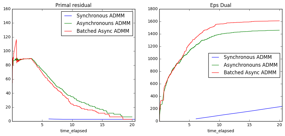
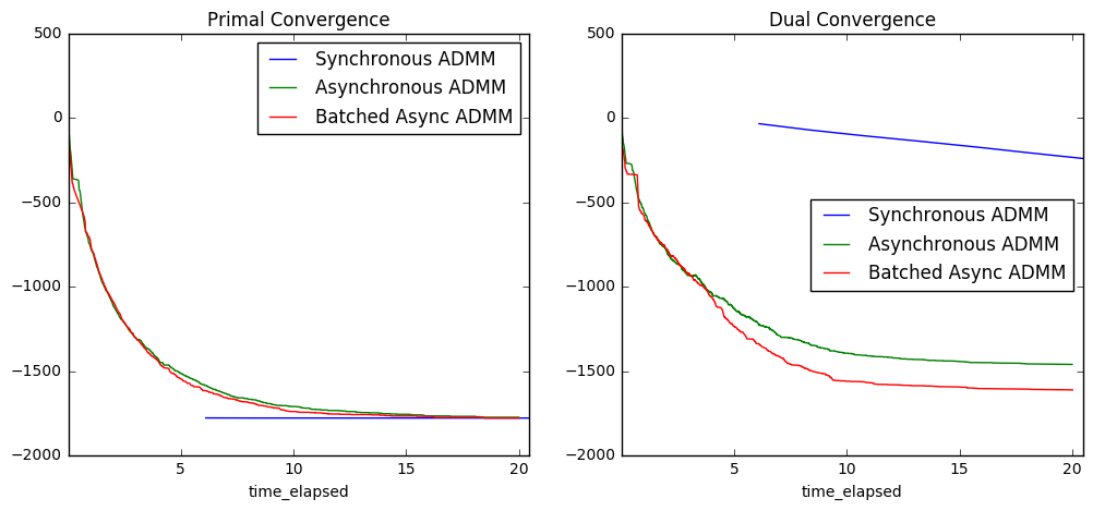
- the primal residual plot measures the amount of disagreement; "small" values imply agreement
- the dual residual plot measures the total "cost" of agreement; this increases until the correct cost is found
The plots then tell us the following:
- the cost of agreement is higher for asynchronous algorithms, which makes sense because each worker is always working with a slightly out-of-date global parameter estimate,
making consensus harder
- blocked ADMM doesn't update at all until shortly after 5 seconds have passed, whereas async has already had time to converge.
(In practice with real data, we would probably specify that all workers need to report in every K updates).
- asynchronous algorithms take a little while for the information to properly diffuse, but once that happens they converge quickly.
- both asynchronous and synchronous converge almost immediately; this is most likely due to a high degree of homogeneity in the data (which was generated to fit the model well). Our next experiment should involve real world data.
## What we could have done better
Analysis wise we expect richer results by performing this same experiment on a real world data set that isn't as homogeneous as the current toy dataset.
Performance wise we can get much better CPU saturation by doing two things:
1. Not running our convergence diagnostics, or making them much faster
2. Not running full `np.mean` computations over all of beta when we've only
updated a few elements. Instead we should maintain a running aggregation
of these results.
With these two changes (each of which are easy) we're fairly confident that we
can scale out to decently large clusters while still saturating hardware.
## Analysis
To get a better sense of what these plots convey, recall that optimization problems always come in pairs: the _primal_ problem
is typically the main problem of interest, and the _dual_ problem is a closely related problem that provides information about
the constraints in the primal problem. Perhaps the most famous example of duality is the [Max-flow-min-cut Theorem](https://en.wikipedia.org/wiki/Max-flow_min-cut_theorem)
from graph theory. In many cases, solving both of these problems simultaneously leads to gains in performance, which is what ADMM seeks to do.
In our case, the constraint in the primal problem is that _all workers must agree on the optimum parameter estimate._ Consequently, we can think
of the dual variables (one for each chunk of data) as measuring the "cost" of agreement for their respective chunks. Intuitively, they will start
out small and grow incrementally to find the right "cost" for each worker to have consensus. Eventually, they will level out at an optimum cost.
So:
- the primal residual plot measures the amount of disagreement; "small" values imply agreement
- the dual residual plot measures the total "cost" of agreement; this increases until the correct cost is found
The plots then tell us the following:
- the cost of agreement is higher for asynchronous algorithms, which makes sense because each worker is always working with a slightly out-of-date global parameter estimate,
making consensus harder
- blocked ADMM doesn't update at all until shortly after 5 seconds have passed, whereas async has already had time to converge.
(In practice with real data, we would probably specify that all workers need to report in every K updates).
- asynchronous algorithms take a little while for the information to properly diffuse, but once that happens they converge quickly.
- both asynchronous and synchronous converge almost immediately; this is most likely due to a high degree of homogeneity in the data (which was generated to fit the model well). Our next experiment should involve real world data.
## What we could have done better
Analysis wise we expect richer results by performing this same experiment on a real world data set that isn't as homogeneous as the current toy dataset.
Performance wise we can get much better CPU saturation by doing two things:
1. Not running our convergence diagnostics, or making them much faster
2. Not running full `np.mean` computations over all of beta when we've only
updated a few elements. Instead we should maintain a running aggregation
of these results.
With these two changes (each of which are easy) we're fairly confident that we
can scale out to decently large clusters while still saturating hardware.