---
blogpost: true
date: Jan 12, 2017
title: Distributed Pandas on a Cluster with Dask DataFrames
tags: Programming, Python, scipy
---
_This work is supported by [Continuum Analytics](http://continuum.io)
the [XDATA Program](http://www.darpa.mil/program/XDATA)
and the Data Driven Discovery Initiative from the [Moore
Foundation](https://www.moore.org/)_
## Summary
Dask Dataframe extends the popular Pandas library to operate on big data-sets
on a distributed cluster. We show its capabilities by running through common
dataframe operations on a common dataset. We break up these computations into
the following sections:
1. Introduction: Pandas is intuitive and fast, but needs Dask to scale
2. Read CSV and Basic operations
1. Read CSV
2. Basic Aggregations and Groupbys
3. Joins and Correlations
3. Shuffles and Time Series
4. Parquet I/O
5. Final thoughts
6. What we could have done better
## Accompanying Plots
Throughout this post we accompany computational examples with profiles of
exactly what task ran where on our cluster and when. These profiles are
interactive [Bokeh plots](https://bokeh.pydata.org) that include every task
that every worker in our cluster runs over time. For example the following
computation `read_csv` computation produces the following profile:
```python
>>> df = dd.read_csv('s3://dask-data/nyc-taxi/2015/*.csv')
```
_If you are reading this through a syndicated website like planet.python.org or
through an RSS reader then these plots will not show up. You may want to visit
[/2017/01/12/dask-dataframes](/2017/01/12/dask-dataframes)
directly._
Dask.dataframe breaks up reading this data into many small tasks of
different types. For example reading bytes and parsing those bytes into
pandas dataframes. Each rectangle corresponds to one task. The y-axis
enumerates each of the worker processes. We have 64 processes spread over
8 machines so there are 64 rows. You can hover over any rectangle to get more
information about that task. You can also use the tools in the upper right
to zoom around and focus on different regions in the computation. In this
computation we can see that workers interleave reading bytes from S3 (light
green) and parsing bytes to dataframes (dark green). The entire computation
took about a minute and most of the workers were busy the entire time (little
white space). Inter-worker communication is always depicted in red (which is
absent in this relatively straightforward computation.)
## Introduction
Pandas provides an intuitive, powerful, and fast data analysis experience on
tabular data. However, because Pandas uses only one thread of execution and
requires all data to be in memory at once, it doesn't scale well to datasets
much beyond the gigabyte scale. That component is missing. Generally people
move to Spark DataFrames on HDFS or a proper relational database to resolve
this scaling issue. Dask is a Python library for parallel and distributed
computing that aims to fill this need for parallelism among the PyData projects
(NumPy, Pandas, Scikit-Learn, etc.). Dask dataframes combine Dask and Pandas
to deliver a faithful "big data" version of Pandas operating in parallel over a
cluster.
[I've written about this topic
before](/2016/02/22/dask-distributed-part-2).
This blogpost is newer and will focus on performance and newer features like
fast shuffles and the Parquet format.
## CSV Data and Basic Operations
I have an eight node cluster on EC2 of `m4.2xlarges` (eight cores, 30GB RAM each).
Dask is running on each node with one process per core.
We have the [2015 Yellow Cab NYC Taxi
data](http://www.nyc.gov/html/tlc/html/about/trip_record_data.shtml) as 12 CSV
files on S3. We look at that data briefly with
[s3fs](http://s3fs.readthedocs.io/en/latest/)
```python
>>> import s3fs
>>> s3 = S3FileSystem()
>>> s3.ls('dask-data/nyc-taxi/2015/')
['dask-data/nyc-taxi/2015/yellow_tripdata_2015-01.csv',
'dask-data/nyc-taxi/2015/yellow_tripdata_2015-02.csv',
'dask-data/nyc-taxi/2015/yellow_tripdata_2015-03.csv',
'dask-data/nyc-taxi/2015/yellow_tripdata_2015-04.csv',
'dask-data/nyc-taxi/2015/yellow_tripdata_2015-05.csv',
'dask-data/nyc-taxi/2015/yellow_tripdata_2015-06.csv',
'dask-data/nyc-taxi/2015/yellow_tripdata_2015-07.csv',
'dask-data/nyc-taxi/2015/yellow_tripdata_2015-08.csv',
'dask-data/nyc-taxi/2015/yellow_tripdata_2015-09.csv',
'dask-data/nyc-taxi/2015/yellow_tripdata_2015-10.csv',
'dask-data/nyc-taxi/2015/yellow_tripdata_2015-11.csv',
'dask-data/nyc-taxi/2015/yellow_tripdata_2015-12.csv']
```
This data is too large to fit into Pandas on a single computer. However, it
can fit in memory if we break it up into many small pieces and load these
pieces onto different computers across a cluster.
We connect a client to our Dask cluster, composed of one centralized
`dask-scheduler` process and several `dask-worker` processes running on each of the
machines in our cluster.
```python
from dask.distributed import Client
client = Client('scheduler-address:8786')
```
And we load our CSV data using `dask.dataframe` which looks and feels just
like Pandas, even though it's actually coordinating hundreds of small Pandas
dataframes. This takes about a minute to load and parse.
```python
import dask.dataframe as dd
df = dd.read_csv('s3://dask-data/nyc-taxi/2015/*.csv',
parse_dates=['tpep_pickup_datetime', 'tpep_dropoff_datetime'],
storage_options={'anon': True})
df = client.persist(df)
```
This cuts up our 12 CSV files on S3 into a few hundred blocks of bytes, each
64MB large. On each of these 64MB blocks we then call `pandas.read_csv` to
create a few hundred Pandas dataframes across our cluster, one for each block
of bytes. Our single Dask Dataframe object, `df`, coordinates all of those
Pandas dataframes. Because we're just using Pandas calls it's very easy for
Dask dataframes to use all of the tricks from Pandas. For example we can use
most of the keyword arguments from `pd.read_csv` in `dd.read_csv` without
having to relearn anything.
This data is about 20GB on disk or 60GB in RAM. It's not huge, but is also
larger than we'd like to manage on a laptop, especially if we value
interactivity. The interactive image above is a trace over time of what each
of our 64 cores was doing at any given moment. By hovering your mouse over the
rectangles you can see that cores switched between downloading byte ranges from
S3 and parsing those bytes with `pandas.read_csv`.
Our dataset includes every cab ride in the city of New York in the year of
2015, including when and where it started and stopped, a breakdown of the fare,
etc.
```python
>>> df.head()
```
|
VendorID |
tpep_pickup_datetime |
tpep_dropoff_datetime |
passenger_count |
trip_distance |
pickup_longitude |
pickup_latitude |
RateCodeID |
store_and_fwd_flag |
dropoff_longitude |
dropoff_latitude |
payment_type |
fare_amount |
extra |
mta_tax |
tip_amount |
tolls_amount |
improvement_surcharge |
total_amount |
| 0 |
2 |
2015-01-15 19:05:39 |
2015-01-15 19:23:42 |
1 |
1.59 |
-73.993896 |
40.750111 |
1 |
N |
-73.974785 |
40.750618 |
1 |
12.0 |
1.0 |
0.5 |
3.25 |
0.0 |
0.3 |
17.05 |
| 1 |
1 |
2015-01-10 20:33:38 |
2015-01-10 20:53:28 |
1 |
3.30 |
-74.001648 |
40.724243 |
1 |
N |
-73.994415 |
40.759109 |
1 |
14.5 |
0.5 |
0.5 |
2.00 |
0.0 |
0.3 |
17.80 |
| 2 |
1 |
2015-01-10 20:33:38 |
2015-01-10 20:43:41 |
1 |
1.80 |
-73.963341 |
40.802788 |
1 |
N |
-73.951820 |
40.824413 |
2 |
9.5 |
0.5 |
0.5 |
0.00 |
0.0 |
0.3 |
10.80 |
| 3 |
1 |
2015-01-10 20:33:39 |
2015-01-10 20:35:31 |
1 |
0.50 |
-74.009087 |
40.713818 |
1 |
N |
-74.004326 |
40.719986 |
2 |
3.5 |
0.5 |
0.5 |
0.00 |
0.0 |
0.3 |
4.80 |
| 4 |
1 |
2015-01-10 20:33:39 |
2015-01-10 20:52:58 |
1 |
3.00 |
-73.971176 |
40.762428 |
1 |
N |
-74.004181 |
40.742653 |
2 |
15.0 |
0.5 |
0.5 |
0.00 |
0.0 |
0.3 |
16.30 |
### Basic Aggregations and Groupbys
As a quick exercise, we compute the length of the dataframe. When we call
`len(df)` Dask.dataframe translates this into many `len` calls on each of the
constituent Pandas dataframes, followed by communication of the intermediate
results to one node, followed by a `sum` of all of the intermediate lengths.
```python
>>> len(df)
146112989
```
This takes around 400-500ms. You can see that a few hundred length
computations happened quickly on the left, followed by some delay, then a bit
of data transfer (the red bar in the plot), and a final summation call.
More complex operations like simple groupbys look similar, although sometimes
with more communications. Throughout this post we're going to do more and more
complex computations and our profiles will similarly become more and more rich
with information. Here we compute the average trip distance, grouped by number
of passengers. We find that single and double person rides go far longer
distances on average. We acheive this one big-data-groupby by performing many
small Pandas groupbys and then cleverly combining their results.
```python
>>> df.groupby(df.passenger_count).trip_distance.mean().compute()
passenger_count
0 2.279183
1 15.541413
2 11.815871
3 1.620052
4 7.481066
5 3.066019
6 2.977158
9 5.459763
7 3.303054
8 3.866298
Name: trip_distance, dtype: float64
```
As a more complex operation we see how well New Yorkers tip by hour of day and
by day of week.
```python
df2 = df[(df.tip_amount > 0) & (df.fare_amount > 0)] # filter out bad rows
df2['tip_fraction'] = df2.tip_amount / df2.fare_amount # make new column
dayofweek = (df2.groupby(df2.tpep_pickup_datetime.dt.dayofweek)
.tip_fraction
.mean())
hour = (df2.groupby(df2.tpep_pickup_datetime.dt.hour)
.tip_fraction
.mean())
```
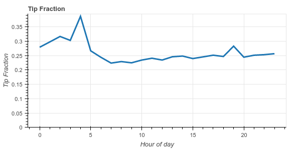 We see that New Yorkers are generally pretty generous, tipping around 20%-25%
on average. We also notice that they become _very generous_ at 4am, tipping an
average of 38%.
This more complex operation uses more of the Dask dataframe API (which mimics
the Pandas API). Pandas users should find the code above fairly familiar. We
remove rows with zero fare or zero tip (not every tip gets recorded), make a
new column which is the ratio of the tip amount to the fare amount, and then
groupby the day of week and hour of day, computing the average tip fraction for
each hour/day.
Dask evaluates this computation with thousands of small Pandas calls across the
cluster (try clicking the wheel zoom icon in the upper right of the image
above and zooming in). The answer comes back in about 3 seconds.
### Joins and Correlations
To show off more basic functionality we'll join this Dask dataframe against a
smaller Pandas dataframe that includes names of some of the more cryptic
columns. Then we'll correlate two derived columns to determine if there is a
relationship between paying Cash and the recorded tip.
```python
>>> payments = pd.Series({1: 'Credit Card',
2: 'Cash',
3: 'No Charge',
4: 'Dispute',
5: 'Unknown',
6: 'Voided trip'})
>>> df2 = df.merge(payments, left_on='payment_type', right_index=True)
>>> df2.groupby(df2.payment_name).tip_amount.mean().compute()
payment_name
Cash 0.000217
Credit Card 2.757708
Dispute -0.011553
No charge 0.003902
Unknown 0.428571
Name: tip_amount, dtype: float64
```
We see that while the average tip for a credit card transaction is $2.75, the
average tip for a cash transaction is very close to zero. At first glance it
seems like cash tips aren't being reported. To investigate this a bit further
lets compute the Pearson correlation between paying cash and having zero tip.
Again, this code should look very familiar to Pandas users.
```python
zero_tip = df2.tip_amount == 0
cash = df2.payment_name == 'Cash'
dd.concat([zero_tip, cash], axis=1).corr().compute()
```
We see that New Yorkers are generally pretty generous, tipping around 20%-25%
on average. We also notice that they become _very generous_ at 4am, tipping an
average of 38%.
This more complex operation uses more of the Dask dataframe API (which mimics
the Pandas API). Pandas users should find the code above fairly familiar. We
remove rows with zero fare or zero tip (not every tip gets recorded), make a
new column which is the ratio of the tip amount to the fare amount, and then
groupby the day of week and hour of day, computing the average tip fraction for
each hour/day.
Dask evaluates this computation with thousands of small Pandas calls across the
cluster (try clicking the wheel zoom icon in the upper right of the image
above and zooming in). The answer comes back in about 3 seconds.
### Joins and Correlations
To show off more basic functionality we'll join this Dask dataframe against a
smaller Pandas dataframe that includes names of some of the more cryptic
columns. Then we'll correlate two derived columns to determine if there is a
relationship between paying Cash and the recorded tip.
```python
>>> payments = pd.Series({1: 'Credit Card',
2: 'Cash',
3: 'No Charge',
4: 'Dispute',
5: 'Unknown',
6: 'Voided trip'})
>>> df2 = df.merge(payments, left_on='payment_type', right_index=True)
>>> df2.groupby(df2.payment_name).tip_amount.mean().compute()
payment_name
Cash 0.000217
Credit Card 2.757708
Dispute -0.011553
No charge 0.003902
Unknown 0.428571
Name: tip_amount, dtype: float64
```
We see that while the average tip for a credit card transaction is $2.75, the
average tip for a cash transaction is very close to zero. At first glance it
seems like cash tips aren't being reported. To investigate this a bit further
lets compute the Pearson correlation between paying cash and having zero tip.
Again, this code should look very familiar to Pandas users.
```python
zero_tip = df2.tip_amount == 0
cash = df2.payment_name == 'Cash'
dd.concat([zero_tip, cash], axis=1).corr().compute()
```
|
tip_amount |
payment_name |
| tip_amount |
1.000000 |
0.943123 |
| payment_name |
0.943123 |
1.000000 |
So we see that standard operations like row filtering, column selection,
groupby-aggregations, joining with a Pandas dataframe, correlations, etc. all
look and feel like the Pandas interface. Additionally, we've seen through
profile plots that most of the time is spent just running Pandas functions on
our workers, so Dask.dataframe is, in most cases, adding relatively little
overhead. These little functions represented by the rectangles in these plots
are _just pandas functions_. For example the plot above has many rectangles
labeled `merge` if you hover over them. This is just the standard
`pandas.merge` function that we love and know to be very fast in memory.
## Shuffles and Time Series
Distributed dataframe experts will know that none of the operations above
require a _shuffle_. That is we can do most of our work with relatively little
inter-node communication. However not all operations can avoid communication
like this and sometimes we need to exchange most of the data between different
workers.
For example if our dataset is sorted by customer ID but we want to sort it by
time then we need to collect all the rows for January over to one Pandas
dataframe, all the rows for February over to another, etc.. This operation is
called a shuffle and is the base of computations like groupby-apply,
distributed joins on columns that are not the index, etc..
You can do a lot with dask.dataframe without performing shuffles, but sometimes
it's necessary. In the following example we sort our data by pickup datetime.
This will allow fast lookups, fast joins, and fast time series operations, all
common cases. We do one shuffle ahead of time to make all future computations
fast.
We set the index as the pickup datetime column. This takes anywhere from
25-40s and is largely network bound (60GB, some text, eight machines with
eight cores each on AWS non-enhanced network). This also requires running
something like 16000 tiny tasks on the cluster. It's worth zooming in on the
plot below.
```python
>>> df = c.persist(df.set_index('tpep_pickup_datetime'))
```
This operation is expensive, far more expensive than it was with Pandas when
all of the data was in the same memory space on the same computer. This is a
good time to point out that you should only use distributed tools like
Dask.datframe and Spark after tools like Pandas break down. We should only
move to distributed systems when absolutely necessary. However, when it does
become necessary, it's nice knowing that Dask.dataframe can faithfully execute
Pandas operations, even if some of them take a bit longer.
As a result of this shuffle our data is now nicely sorted by time, which will
keep future operations close to optimal. We can see how the dataset is sorted
by pickup time by quickly looking at the first entries, last entries, and
entries for a particular day.
```python
>>> df.head() # has the first entries of 2015
```
|
VendorID |
tpep_dropoff_datetime |
passenger_count |
trip_distance |
pickup_longitude |
pickup_latitude |
RateCodeID |
store_and_fwd_flag |
dropoff_longitude |
dropoff_latitude |
payment_type |
fare_amount |
extra |
mta_tax |
tip_amount |
tolls_amount |
improvement_surcharge |
total_amount |
| tpep_pickup_datetime |
|
|
|
|
|
|
|
|
|
|
|
|
|
|
|
|
|
|
| 2015-01-01 00:00:00 |
2 |
2015-01-01 00:00:00 |
3 |
1.56 |
-74.001320 |
40.729057 |
1 |
N |
-74.010208 |
40.719662 |
1 |
7.5 |
0.5 |
0.5 |
0.0 |
0.0 |
0.3 |
8.8 |
| 2015-01-01 00:00:00 |
2 |
2015-01-01 00:00:00 |
1 |
1.68 |
-73.991547 |
40.750069 |
1 |
N |
0.000000 |
0.000000 |
2 |
10.0 |
0.0 |
0.5 |
0.0 |
0.0 |
0.3 |
10.8 |
| 2015-01-01 00:00:00 |
1 |
2015-01-01 00:11:26 |
5 |
4.00 |
-73.971436 |
40.760201 |
1 |
N |
-73.921181 |
40.768269 |
2 |
13.5 |
0.5 |
0.5 |
0.0 |
0.0 |
0.0 |
14.5 |
```python
>>> df.tail() # has the last entries of 2015
```
|
VendorID |
tpep_dropoff_datetime |
passenger_count |
trip_distance |
pickup_longitude |
pickup_latitude |
RateCodeID |
store_and_fwd_flag |
dropoff_longitude |
dropoff_latitude |
payment_type |
fare_amount |
extra |
mta_tax |
tip_amount |
tolls_amount |
improvement_surcharge |
total_amount |
| tpep_pickup_datetime |
|
|
|
|
|
|
|
|
|
|
|
|
|
|
|
|
|
|
| 2015-12-31 23:59:56 |
1 |
2016-01-01 00:09:25 |
1 |
1.00 |
-73.973900 |
40.742893 |
1 |
N |
-73.989571 |
40.750549 |
1 |
8.0 |
0.5 |
0.5 |
1.85 |
0.0 |
0.3 |
11.15 |
| 2015-12-31 23:59:58 |
1 |
2016-01-01 00:05:19 |
2 |
2.00 |
-73.965271 |
40.760281 |
1 |
N |
-73.939514 |
40.752388 |
2 |
7.5 |
0.5 |
0.5 |
0.00 |
0.0 |
0.3 |
8.80 |
| 2015-12-31 23:59:59 |
2 |
2016-01-01 00:10:26 |
1 |
1.96 |
-73.997559 |
40.725693 |
1 |
N |
-74.017120 |
40.705322 |
2 |
8.5 |
0.5 |
0.5 |
0.00 |
0.0 |
0.3 |
9.80 |
```python
>>> df.loc['2015-05-05'].head() # has the entries for just May 5th
```
|
VendorID |
tpep_dropoff_datetime |
passenger_count |
trip_distance |
pickup_longitude |
pickup_latitude |
RateCodeID |
store_and_fwd_flag |
dropoff_longitude |
dropoff_latitude |
payment_type |
fare_amount |
extra |
mta_tax |
tip_amount |
tolls_amount |
improvement_surcharge |
total_amount |
| tpep_pickup_datetime |
|
|
|
|
|
|
|
|
|
|
|
|
|
|
|
|
|
|
| 2015-05-05 |
2 |
2015-05-05 00:00:00 |
1 |
1.20 |
-73.981941 |
40.766460 |
1 |
N |
-73.972771 |
40.758007 |
2 |
6.5 |
1.0 |
0.5 |
0.00 |
0.00 |
0.3 |
8.30 |
| 2015-05-05 |
1 |
2015-05-05 00:10:12 |
1 |
1.70 |
-73.994675 |
40.750507 |
1 |
N |
-73.980247 |
40.738560 |
1 |
9.0 |
0.5 |
0.5 |
2.57 |
0.00 |
0.3 |
12.87 |
| 2015-05-05 |
1 |
2015-05-05 00:07:50 |
1 |
2.50 |
-74.002930 |
40.733681 |
1 |
N |
-74.013603 |
40.702362 |
2 |
9.5 |
0.5 |
0.5 |
0.00 |
0.00 |
0.3 |
10.80 |
Because we know exactly which Pandas dataframe holds which data we can
execute row-local queries like this very quickly. The total round trip from
pressing enter in the interpreter or notebook is about 40ms. For reference,
40ms is the delay between two frames in a movie running at 25 Hz. This means
that it's fast enough that human users perceive this query to be entirely
fluid.
### Time Series
Additionally, once we have a nice datetime index all of Pandas' time series
functionality becomes available to us.
For example we can resample by day:
```python
>>> (df.passenger_count
.resample('1d')
.mean()
.compute()
.plot())
```
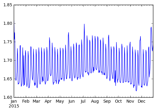 We observe a strong periodic signal here. The number of passengers is reliably
higher on the weekends.
We can perform a rolling aggregation in about a second:
```python
>>> s = client.persist(df.passenger_count.rolling(10).mean())
```
Because Dask.dataframe inherits the Pandas index all of these operations become
very fast and intuitive.
## Parquet
Pandas' standard "fast" recommended storage solution has generally been the
HDF5 data format. Unfortunately the HDF5 file format is not ideal for
distributed computing, so most Dask dataframe users have had to switch down to
CSV historically. This is unfortunate because CSV is slow, doesn't support
partial queries (you can't read in just one column), and also isn't supported
well by the other standard distributed Dataframe solution, Spark. This makes it
hard to move data back and forth.
Fortunately there are now two decent Python readers for Parquet, a fast
columnar binary store that shards nicely on distributed data stores like the
Hadoop File System (HDFS, not to be confused with HDF5) and Amazon's S3. The
already fast [Parquet-cpp project](https://github.com/apache/parquet-cpp) has
been growing Python and Pandas support through
[Arrow](http://pyarrow.readthedocs.io/en/latest/), and the [Fastparquet
project](http://fastparquet.readthedocs.io/), which is an offshoot from the
[pure-python `parquet` library](https://github.com/jcrobak/parquet-python) has
been growing speed through use of
[NumPy](https://docs.scipy.org/doc/numpy/reference/) and
[Numba](http://numba.pydata.org/).
Using Fastparquet under the hood, Dask.dataframe users can now happily read and
write to Parquet files. This increases speed, decreases storage costs, and
provides a shared format that both Dask dataframes and Spark dataframes can
understand, improving the ability to use both computational systems in the same
workflow.
Writing our Dask dataframe to S3 can be as simple as the following:
```python
df.to_parquet('s3://dask-data/nyc-taxi/tmp/parquet')
```
However there are also a variety of options we can use to store our data more
compactly through compression, encodings, etc.. Expert users will probably
recognize some of the terms below.
```python
df = df.astype({'VendorID': 'uint8',
'passenger_count': 'uint8',
'RateCodeID': 'uint8',
'payment_type': 'uint8'})
df.to_parquet('s3://dask-data/nyc-taxi/tmp/parquet',
compression='snappy',
has_nulls=False,
object_encoding='utf8',
fixed_text={'store_and_fwd_flag': 1})
```
We can then read our nicely indexed dataframe back with the
`dd.read_parquet` function:
```python
>>> df2 = dd.read_parquet('s3://dask-data/nyc-taxi/tmp/parquet')
```
The main benefit here is that we can quickly compute on single columns. The
following computation runs in around 6 seconds, even though we don't have any
data in memory to start (recall that we started this blogpost with a
minute-long call to `read_csv`.and
[Client.persist](http://distributed.readthedocs.io/en/latest/api.html#distributed.client.Client.persist))
```python
>>> df2.passenger_count.value_counts().compute()
1 102991045
2 20901372
5 7939001
3 6135107
6 5123951
4 2981071
0 40853
7 239
8 181
9 169
Name: passenger_count, dtype: int64
```
## Final Thoughts
With the recent addition of faster shuffles and Parquet support, Dask
dataframes become significantly more attractive. This blogpost gave a few
categories of common computations, along with precise profiles of their
execution on a small cluster. Hopefully people find this combination of Pandas
syntax and scalable computing useful.
Now would also be a good time to remind people that Dask dataframe is only one
module among many within the [Dask project](http://dask.pydata.org/en/latest/).
Dataframes are nice, certainly, but Dask's main strength is its flexibility to
move beyond just plain dataframe computations to handle even more complex
problems.
## Learn More
If you'd like to learn more about Dask dataframe, the Dask distributed system,
or other components you should look at the following documentation:
1. [http://dask.pydata.org/en/latest/](http://dask.pydata.org/en/latest/)
2. [http://distributed.readthedocs.io/en/latest/](http://distributed.readthedocs.io/en/latest/)
The workflows presented here are captured in the following notebooks (among
other examples):
1. [NYC Taxi example, shuffling, others](https://gist.github.com/mrocklin/ada85ef06d625947f7b34886fd2710f8)
2. [Parquet](https://gist.github.com/mrocklin/89bccf2f4f37611b40c18967bb182066)
## What we could have done better
As always with computational posts we include a section on what went wrong, or
what could have gone better.
1. The 400ms computation of `len(df)` is a regression from previous
versions where this was closer to 100ms. We're getting bogged down
somewhere in many small inter-worker communications.
2. It would be nice to repeat this computation at a larger scale. Dask
deployments in the wild are often closer to 1000 cores rather than the 64
core cluster we have here and datasets are often in the terrabyte scale
rather than our 60 GB NYC Taxi dataset. Unfortunately representative large
open datasets are hard to find.
3. The Parquet timings are nice, but there is still room for improvement. We
seem to be making many small expensive queries of S3 when reading Thrift
headers.
4. It would be nice to support both Python Parquet readers, both the
[Numba](http://numba.pydata.org/) solution
[fastparquet](https://fastparquet.readthedocs.io) and the C++ solution
[parquet-cpp](https://github.com/apache/parquet-cpp)
We observe a strong periodic signal here. The number of passengers is reliably
higher on the weekends.
We can perform a rolling aggregation in about a second:
```python
>>> s = client.persist(df.passenger_count.rolling(10).mean())
```
Because Dask.dataframe inherits the Pandas index all of these operations become
very fast and intuitive.
## Parquet
Pandas' standard "fast" recommended storage solution has generally been the
HDF5 data format. Unfortunately the HDF5 file format is not ideal for
distributed computing, so most Dask dataframe users have had to switch down to
CSV historically. This is unfortunate because CSV is slow, doesn't support
partial queries (you can't read in just one column), and also isn't supported
well by the other standard distributed Dataframe solution, Spark. This makes it
hard to move data back and forth.
Fortunately there are now two decent Python readers for Parquet, a fast
columnar binary store that shards nicely on distributed data stores like the
Hadoop File System (HDFS, not to be confused with HDF5) and Amazon's S3. The
already fast [Parquet-cpp project](https://github.com/apache/parquet-cpp) has
been growing Python and Pandas support through
[Arrow](http://pyarrow.readthedocs.io/en/latest/), and the [Fastparquet
project](http://fastparquet.readthedocs.io/), which is an offshoot from the
[pure-python `parquet` library](https://github.com/jcrobak/parquet-python) has
been growing speed through use of
[NumPy](https://docs.scipy.org/doc/numpy/reference/) and
[Numba](http://numba.pydata.org/).
Using Fastparquet under the hood, Dask.dataframe users can now happily read and
write to Parquet files. This increases speed, decreases storage costs, and
provides a shared format that both Dask dataframes and Spark dataframes can
understand, improving the ability to use both computational systems in the same
workflow.
Writing our Dask dataframe to S3 can be as simple as the following:
```python
df.to_parquet('s3://dask-data/nyc-taxi/tmp/parquet')
```
However there are also a variety of options we can use to store our data more
compactly through compression, encodings, etc.. Expert users will probably
recognize some of the terms below.
```python
df = df.astype({'VendorID': 'uint8',
'passenger_count': 'uint8',
'RateCodeID': 'uint8',
'payment_type': 'uint8'})
df.to_parquet('s3://dask-data/nyc-taxi/tmp/parquet',
compression='snappy',
has_nulls=False,
object_encoding='utf8',
fixed_text={'store_and_fwd_flag': 1})
```
We can then read our nicely indexed dataframe back with the
`dd.read_parquet` function:
```python
>>> df2 = dd.read_parquet('s3://dask-data/nyc-taxi/tmp/parquet')
```
The main benefit here is that we can quickly compute on single columns. The
following computation runs in around 6 seconds, even though we don't have any
data in memory to start (recall that we started this blogpost with a
minute-long call to `read_csv`.and
[Client.persist](http://distributed.readthedocs.io/en/latest/api.html#distributed.client.Client.persist))
```python
>>> df2.passenger_count.value_counts().compute()
1 102991045
2 20901372
5 7939001
3 6135107
6 5123951
4 2981071
0 40853
7 239
8 181
9 169
Name: passenger_count, dtype: int64
```
## Final Thoughts
With the recent addition of faster shuffles and Parquet support, Dask
dataframes become significantly more attractive. This blogpost gave a few
categories of common computations, along with precise profiles of their
execution on a small cluster. Hopefully people find this combination of Pandas
syntax and scalable computing useful.
Now would also be a good time to remind people that Dask dataframe is only one
module among many within the [Dask project](http://dask.pydata.org/en/latest/).
Dataframes are nice, certainly, but Dask's main strength is its flexibility to
move beyond just plain dataframe computations to handle even more complex
problems.
## Learn More
If you'd like to learn more about Dask dataframe, the Dask distributed system,
or other components you should look at the following documentation:
1. [http://dask.pydata.org/en/latest/](http://dask.pydata.org/en/latest/)
2. [http://distributed.readthedocs.io/en/latest/](http://distributed.readthedocs.io/en/latest/)
The workflows presented here are captured in the following notebooks (among
other examples):
1. [NYC Taxi example, shuffling, others](https://gist.github.com/mrocklin/ada85ef06d625947f7b34886fd2710f8)
2. [Parquet](https://gist.github.com/mrocklin/89bccf2f4f37611b40c18967bb182066)
## What we could have done better
As always with computational posts we include a section on what went wrong, or
what could have gone better.
1. The 400ms computation of `len(df)` is a regression from previous
versions where this was closer to 100ms. We're getting bogged down
somewhere in many small inter-worker communications.
2. It would be nice to repeat this computation at a larger scale. Dask
deployments in the wild are often closer to 1000 cores rather than the 64
core cluster we have here and datasets are often in the terrabyte scale
rather than our 60 GB NYC Taxi dataset. Unfortunately representative large
open datasets are hard to find.
3. The Parquet timings are nice, but there is still room for improvement. We
seem to be making many small expensive queries of S3 when reading Thrift
headers.
4. It would be nice to support both Python Parquet readers, both the
[Numba](http://numba.pydata.org/) solution
[fastparquet](https://fastparquet.readthedocs.io) and the C++ solution
[parquet-cpp](https://github.com/apache/parquet-cpp)